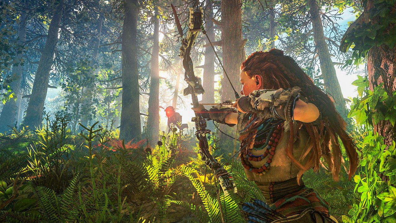
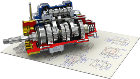
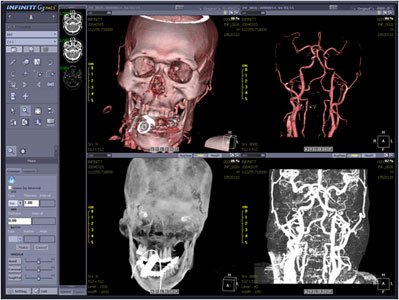
Exemples d'applications 3D : jeu vidéo (gauche), CAO (centre), imagerie médicale (droite).
3D models are ubiquitous in many fields:
Some examples of these applications are presented below.
Exemples d'applications 3D : jeu vidéo (gauche), CAO (centre), imagerie médicale (droite).
The creation and manipulation of 3D content remain, however, complex and costly:
Generative AI-based automatic tools are beginning to emerge, but remain highly difficult to control and with a significant environmental cost. They are still largely experimental for real-world productions. Controllability, quality, and efficiency remain major challenges.
The computer graphics (Computer Graphics) designates the set of sciences and techniques enabling the generation and manipulation of visual data:
Applications are numerous: entertainment, design, simulation of natural phenomena, medical, biological, etc.
Computer graphics is structured around three major domains :
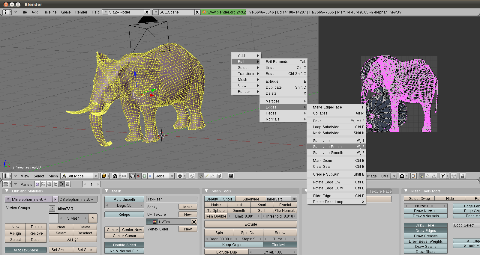
Modeling (Modeling) : creation and representation of 3D shapes. This covers the design of the geometry of objects (their shape, their structure) as well as their visual attributes (textures, materials). Modeling can be manual (an artist using software such as Blender or Maya) or procedural (algorithmic generation of shapes).
Animation : moving objects and characters over time. Animation encompasses both cinematic techniques (explicit movement of objects frame-by-frame or by interpolation of key poses) and physical techniques (simulation of forces, gravity, collisions, fluids, cloth, etc., which automatically generate motion from physical laws).
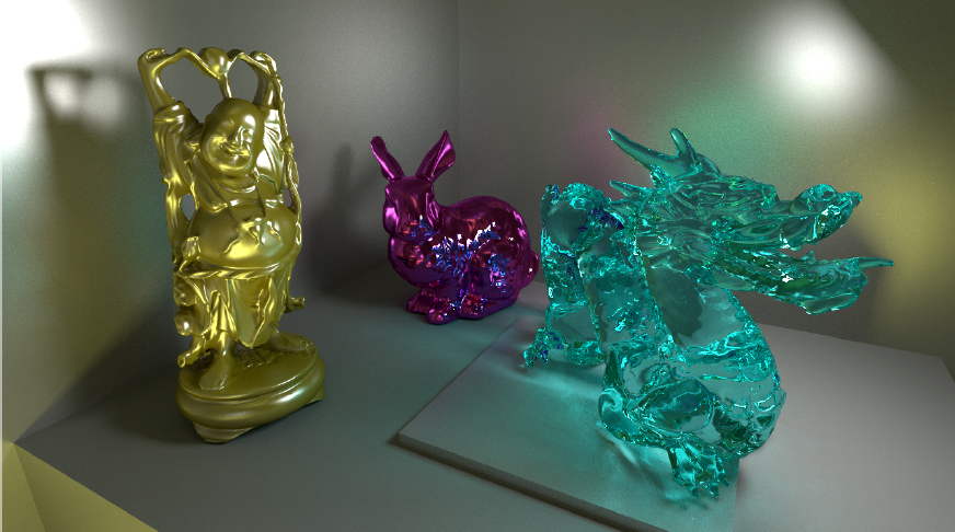
Image Synthesis / Rendering (Rendering) : generation of 2D images from a 3D scene. Rendering takes as input the description of geometry, materials, lights and the camera, then computes the resulting image. One distinguishes the rendering real-time (interactive, typically \(\geq\) 25-60 frames per second, used in video games and visualization) and the rendering offline (photorealistic, potentially taking from a few seconds to several hours per image, used in cinema and architecture).
These three domains are illustrated below.

Modélisation (gauche), animation (centre) et rendu (droite).
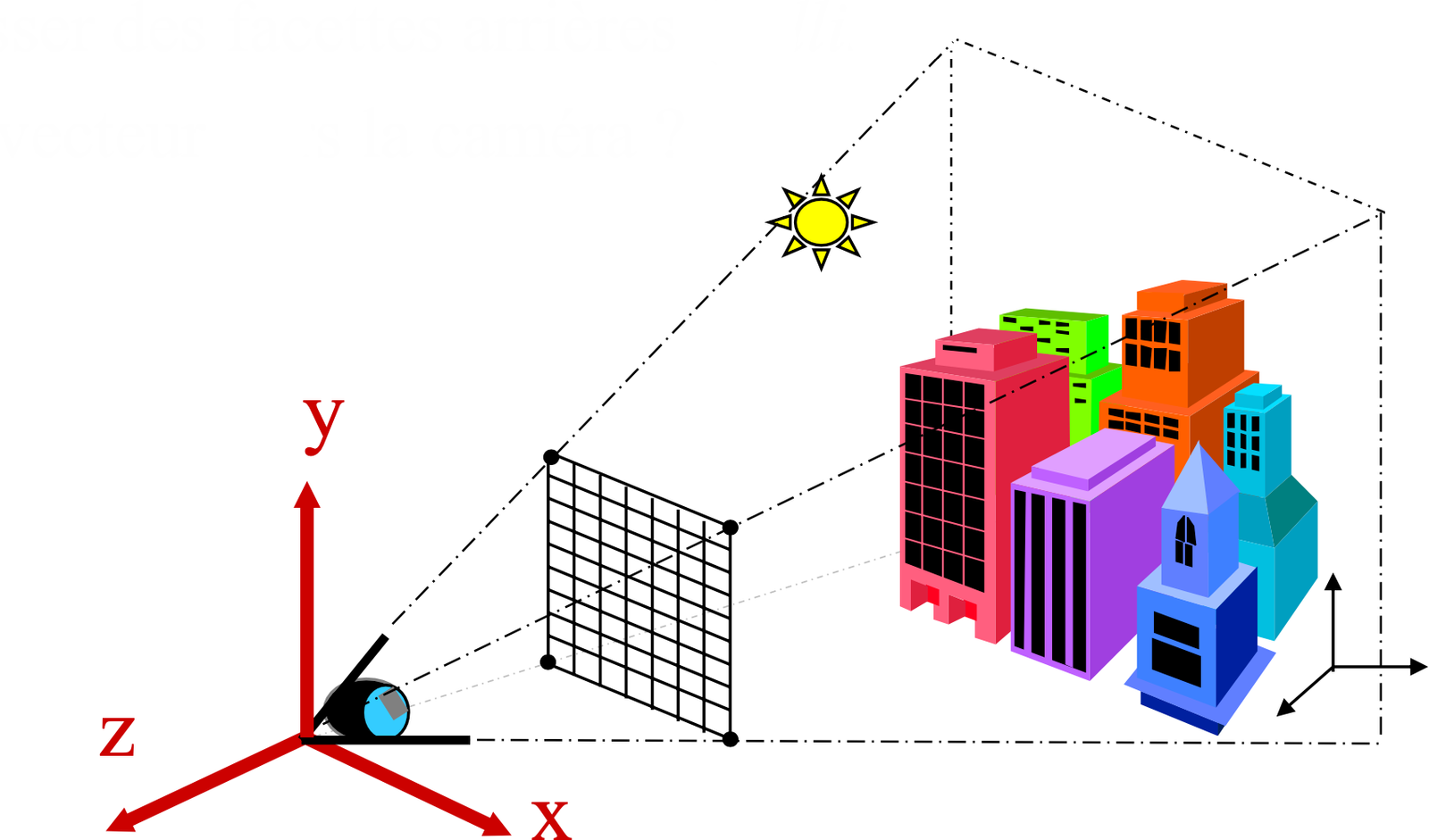
A 3D scene is described by three fundamental components:
3D Model: a surface or a volume representing the objects of the scene. Each object possesses geometry (shape) and visual attributes (color, material, texture). The scene may contain one or more objects, each positioned and oriented in a common 3D space called world space (world space).
Light Source: one or more light sources illuminating the scene. A light source is characterized by its position (or direction), its intensity and its color. Common types include point lights (emission from a point), directional lights (parallel rays, simulating the sun), and area lights (emission from a surface, for softer shadows). The interaction between light and the materials of the objects determines the visual appearance of the scene.
Camera: the viewpoint from which the scene is observed. The camera is defined by its position in space, its orientation (view direction), and its optical parameters (field of view, focal length, aspect ratio). It determines which objects are visible and how they are projected onto the final image.
The output of the rendering process is a 2D image corresponding to what the camera “sees” of the 3D scene. The following diagram summarizes the arrangement of these components.
A fundamental challenge in computer graphics is to give the illusion of depth and volume on a display that is intrinsically a 2D medium. Several visual phenomena contribute to this perception.
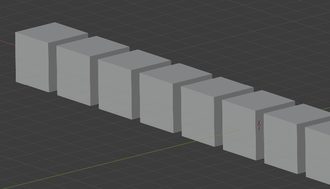
Far objects appear smaller than nearby objects. Two parallel lines in the scene converge toward a vanishing point on the image. This effect is directly related to the perspective projection performed by the camera (see the section on generalized coordinates).
Projection orthographique (gauche) vs projection perspective (droite).
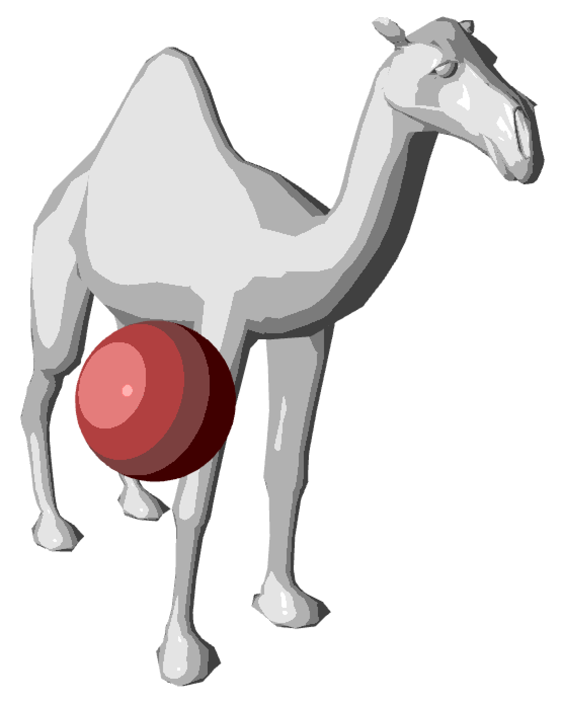
The color of a point on the surface varies according to the orientation of that surface relative to the light source. A surface facing the light appears bright, while a surface turned away from the light appears dark. This gradient of brightness, called shading (shading), provides essential cues about the curvature and volume of objects. By contrast, an object displayed with a uniform color (no shading) appears flat, like a disk rather than a sphere.
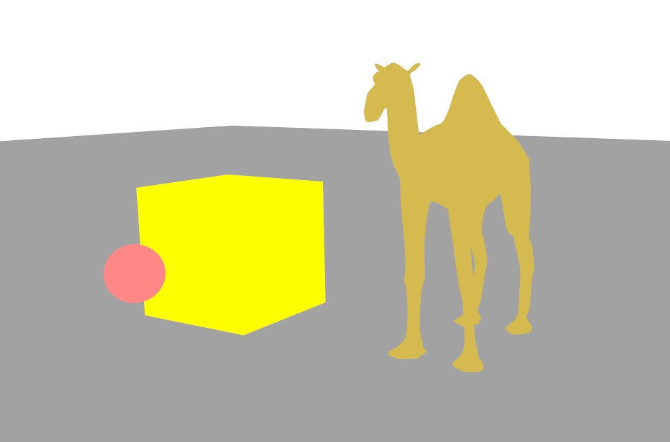
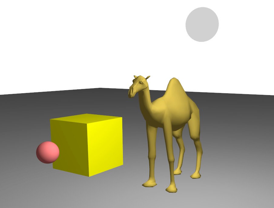
Couleur uniforme (gauche) vs illumination diffuse (droite) : l'ombrage révèle la géométrie.
Nearby objects occlude objects located behind them. This simple yet powerful phenomenon provides a direct cue to the depth ordering of objects in the scene.
The shadow cast by an object onto another object or onto the ground visually anchors the object in the scene and provides information about its relative position and the direction of the light.
An image is a 2D grid of pixels of dimension \(N_x \times N_y\).
Other common formats :
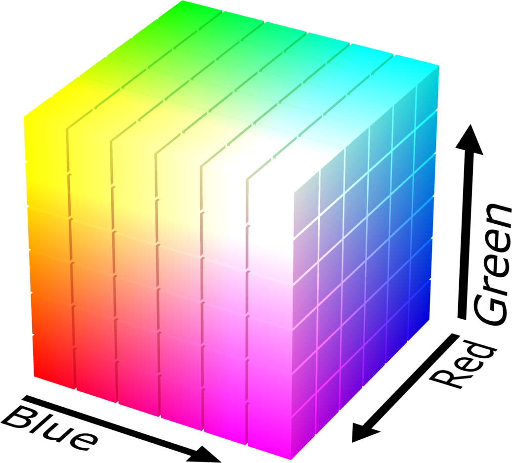
Note : the RGB space is not perceptually uniform (two colors close in RGB distance are not necessarily visually close). The RGB cube is shown in the figure below.
A 3D object can be represented in two fundamental ways:
Volume : complete description of the object, including the interior. For example, one can associate a density, a temperature or any other physical attribute at every point of the volume. This representation is indispensable in medical imaging (MRI, CT scanner), in fluid simulation (smoke, clouds) and in materials physics. However, it is very memory-intensive: a volume with a resolution of \(256^3\) already contains more than 16 million voxels (volumetric pixel).
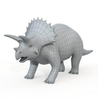
Surface : only the exterior and visible part of the object. Only the “skin” of the object is described, with no information about the interior. This representation is much more memory-efficient and, above all, much more efficient for rendering on the GPU, since only the surface contributes to the final image.
In real-time computer graphics, representations by surface are predominantly used. Volumetric representations are reserved for specific cases (atmospheric effects, medical data, physical simulation). The following figure compares these two approaches.
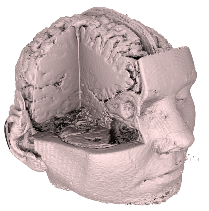
Représentation volumique (gauche) vs représentation surfacique (droite).
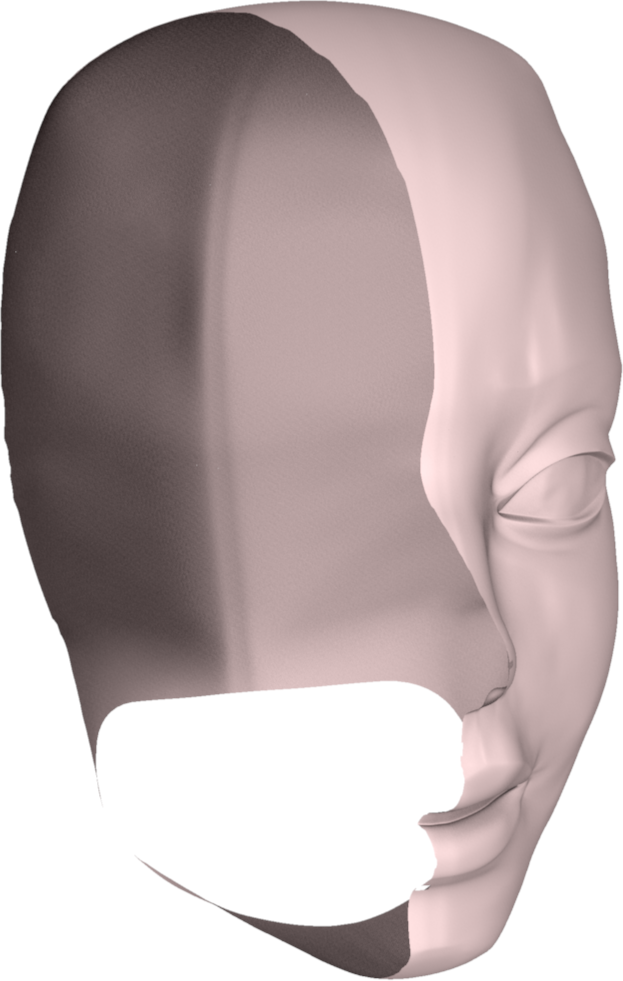
There are two fundamental families of mathematical description of a surface:
The two types of representation are compared in the diagram below.


Surface explicite paramétrique (gauche) vs surface implicite (droite).
In practice, for complex shapes such as a character or a vehicle, no simple analytical formula can describe the surface. We then resort to discrete approximations.
In practice, arbitrary surfaces are rarely described by a single analytic function. Piecewise approximations are used with the aid of primitives and discrete elements.
The ideal properties of a description are:
Examples of models:
Graphics cards are specialized for rendering of triangular meshes.
Ray tracing simulates the physical path of light in the scene. The basic principle is as follows: for each pixel of the image, a ray is cast from the camera through this pixel, and we search for the first object in the scene that this ray intersects. Once the intersection point is found, its color is computed based on the lighting, the material, and possibly reflections and refractions (by recursively launching new rays).
In practice, rays are often traced in the opposite direction of the light (from the camera toward the scene), because the vast majority of rays emitted by a light source never reach the camera. This inverse tracing is much more efficient.
Advantages:
Disadvantages:
The principle is summarized in the following diagram.

The rasterization approach adopts a radically different strategy from ray tracing. Instead of starting from each pixel and searching which object is visible, we start from each object (triangle) and determine which pixels it covers. This approach assumes that the scene is composed of triangles. The process unfolds in two steps:
Projection : each vertex of the triangle is projected from 3D space onto the camera’s 2D plane. This operation is performed by a matrix multiplication in a projective space: \(p' = M \, p\), where \(M\) is the matrix combining the transformation of the scene, the placement of the camera, and the perspective projection. This operation is extremely fast because it reduces to a matrix-vector product per vertex.
Rasterization : once the triangles are projected in 2D, each triangle is “filled” pixel by pixel. For each pixel covered by the triangle, its barycentric coordinates are computed and the attributes of the vertices (color, normal, texture coordinates, etc.) are interpolated to obtain the value at the pixel. Each such pixel is called a fragment.
These two steps are illustrated below.


Projection des sommets sur le plan caméra (gauche) et rasterization des triangles en pixels (droite).
A z-buffer mechanism (depth buffer) handles occlusion: for each pixel, we keep only the fragment closest to the camera, ensuring that objects in front occlude those behind.
Advantages :
Disadvantages :
Rasterization is the real-time rendering standard on GPUs. It is the approach used in all video games, interactive visualization applications and CAD software.
A triangular mesh is the simplest and most widespread representation to approximate a continuous surface by a set of triangles. The more triangles there are, the closer the approximation is to the original surface, but the higher the storage and rendering cost. In practice, a typical 3D model in a video game contains from a few thousand to several hundred thousand triangles. A high-resolution model for cinema can contain several million triangles.
A mesh is described by three types of elements :
 Vertices (vertices) : the 3D points that form the
corners of the triangles. The set of vertices is denoted \(\mathcal{V} = (p_1, \dots, p_{N_v})\) with
\(p_i = (x_i, y_i, z_i) \in
\mathbb{R}^3\). Each vertex can carry additional attributes: a
normal (direction perpendicular to the surface at this point), a color,
texture coordinates, etc.
Vertices (vertices) : the 3D points that form the
corners of the triangles. The set of vertices is denoted \(\mathcal{V} = (p_1, \dots, p_{N_v})\) with
\(p_i = (x_i, y_i, z_i) \in
\mathbb{R}^3\). Each vertex can carry additional attributes: a
normal (direction perpendicular to the surface at this point), a color,
texture coordinates, etc.
 Faces : each face is a triangle defined by a triplet of
vertex indices \(\mathcal{F} = (f_1, \dots,
f_{N_f})\) with \(f_i = (p_{i_1},
p_{i_2}, p_{i_3})\). The faces define the
connectivity (or topology) of the mesh, i.e., how the
vertices are connected to each other.
Faces : each face is a triangle defined by a triplet of
vertex indices \(\mathcal{F} = (f_1, \dots,
f_{N_f})\) with \(f_i = (p_{i_1},
p_{i_2}, p_{i_3})\). The faces define the
connectivity (or topology) of the mesh, i.e., how the
vertices are connected to each other.
 Edges (optional) : segments connecting two adjacent
vertices \(\mathcal{E} = (e_1, \dots,
e_{N_e})\) with \(e_i = (p_{i_1},
p_{i_2})\). Edges are not always stored explicitly as they can be
inferred from the faces, but they are useful for certain algorithms
(subdivision, simplification, etc.).
Edges (optional) : segments connecting two adjacent
vertices \(\mathcal{E} = (e_1, \dots,
e_{N_e})\) with \(e_i = (p_{i_1},
p_{i_2})\). Edges are not always stored explicitly as they can be
inferred from the faces, but they are useful for certain algorithms
(subdivision, simplification, etc.).
Concrete examples of meshes are shown below.
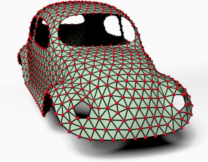
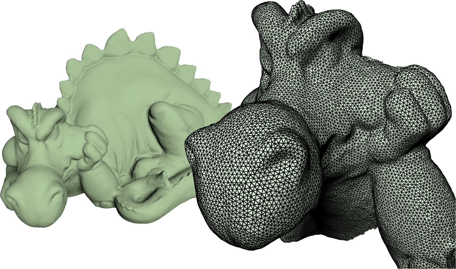
Exemples de maillages triangulaires : modèle de voiture (gauche) et modèle de dragon (droite).
A triangle \(T\) is defined by three vertices \((p_1, p_2, p_3)\). The triangle is the basic element of rasterization and possesses very useful mathematical properties that we detail below.
Every point \(p\) inside the triangle can be expressed as a linear combination of the two edges emanating from \(p_1\):
\[ p \in T \Leftrightarrow S(u,v) = p_1 + u\,(p_2 - p_1) + v\,(p_3 - p_1), \quad u \geq 0, \; v \geq 0, \; u+v \leq 1 \] The parameters \((u,v)\) form a local coordinate system on the triangle. The vertex \(p_1\) corresponds to \((0,0)\), \(p_2\) to \((1,0)\) and \(p_3\) to \((0,1)\).
An equivalent and often more convenient way to parameterize a triangle is to use the barycentric coordinates \((\alpha, \beta, \gamma)\):
\[ p \in T \Leftrightarrow p = \alpha \, p_1 + \beta \, p_2 + \gamma \, p_3, \quad \alpha, \beta, \gamma \in [0,1], \; \alpha + \beta + \gamma = 1 \] Barycentric coordinates have an intuitive geometric interpretation: \(\alpha\) represents the “weight” or the influence of vertex \(p_1\) on the point \(p\). The closer \(p\) is to \(p_1\), the larger \(\alpha\) is (close to 1) and the smaller \(\beta\) and \(\gamma\) are. At the vertices, we have respectively \((\alpha, \beta, \gamma) = (1,0,0)\), \((0,1,0)\) and \((0,0,1)\). At the barycentre of the triangle, the three coordinates equal \(1/3\).
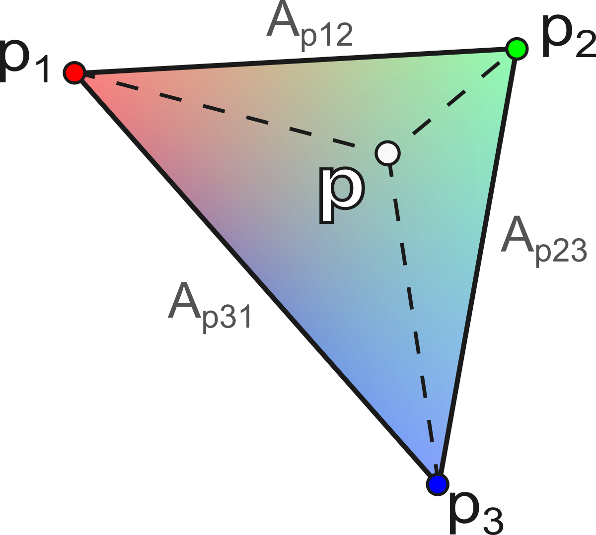
The calculation of barycentric coordinates for a point p is performed via the ratio of the areas of the sub-triangles:
\[ \alpha = \frac{A_{p23}}{A_{123}}, \quad \beta = \frac{A_{p31}}{A_{123}}, \quad \gamma = \frac{A_{p12}}{A_{123}} \] with \(A_{123} = \frac{1}{2} \| (p_2 - p_1) \times (p_3 - p_1) \|\) the total area of the triangle, and \(A_{p23}\), \(A_{p31}\), \(A_{p12}\) the areas of the sub-triangles formed by \(p\) with the opposite edges :
\[ \begin{aligned} A_{p23} &= \tfrac{1}{2} \| (p_2 - p) \times (p_3 - p) \| \\ A_{p31} &= \tfrac{1}{2} \| (p_3 - p) \times (p_1 - p) \| \\ A_{p12} &= \tfrac{1}{2} \| (p_1 - p) \times (p_2 - p) \| \end{aligned} \] This geometric construction is illustrated in the figure below.
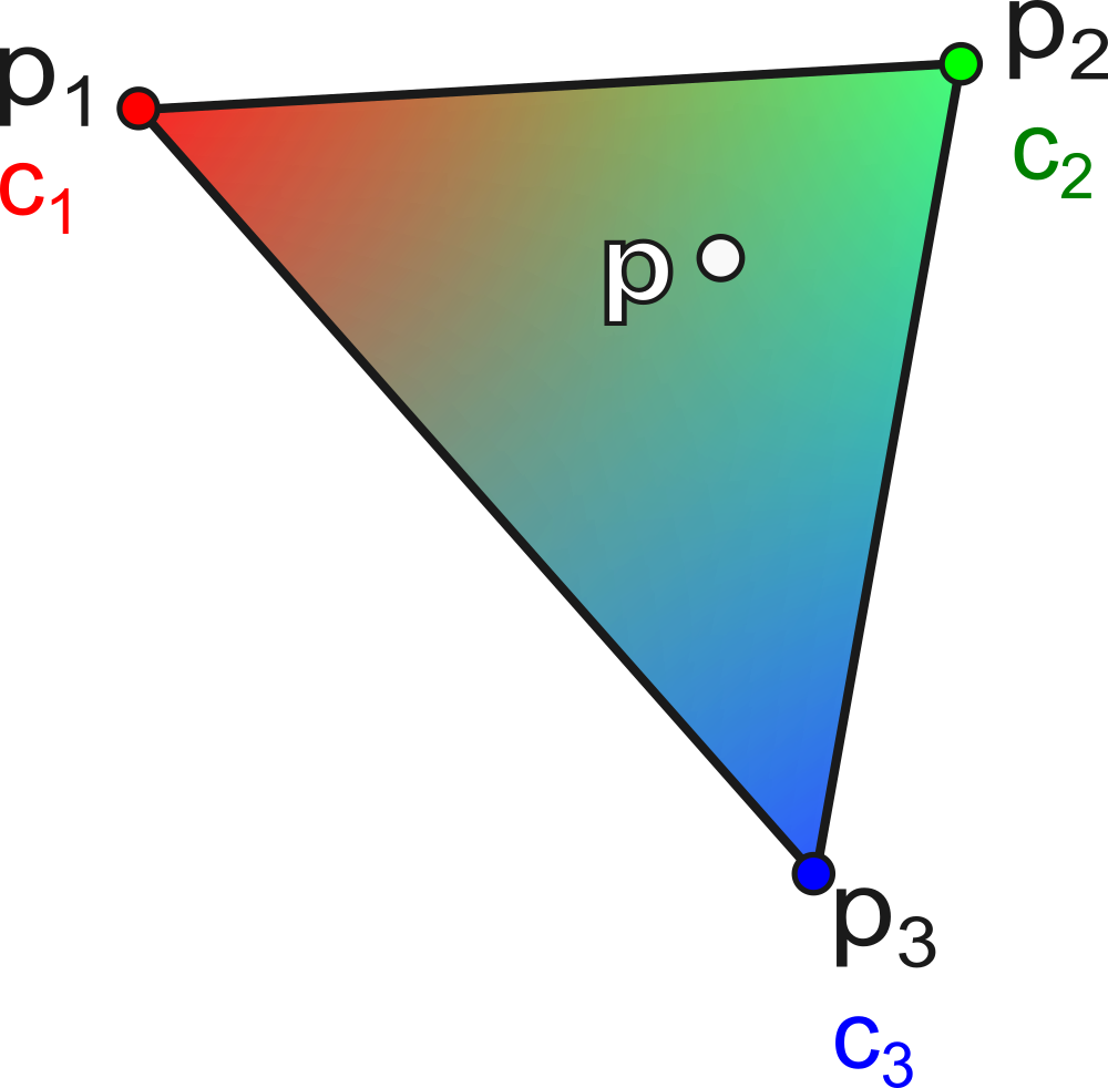
Let a triangle \(T\) with colors \((c_1, c_2, c_3)\) associated with the vertices \((p_1, p_2, p_3)\). The interpolated color at a point \(p\) inside the triangle is:
\[ c(p) = \alpha \, c_1 + \beta \, c_2 + \gamma \, c_3 \] where \((\alpha, \beta, \gamma)\) are the barycentric coordinates of \(p\).
This interpolation is fundamental in rendering: it is used to interpolate colors, normals, texture coordinates, etc., inside each triangle. An example of color interpolation is shown below.
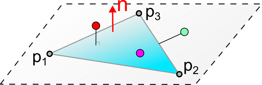
To test whether a point \(p\) is inside a triangle \(T = (p_1, p_2, p_3)\):
Necessary condition: \(p\) must lie in the plane of the triangle. We verify that \((p - p_1) \cdot n = 0\) with \(n = (p_2 - p_1) \times (p_3 - p_1)\) (normal to the triangle).
Sufficient condition: calculation of barycentric coordinates \((\alpha, \beta, \gamma)\). We verify that \(0 \leq \alpha, \beta, \gamma \leq 1\) and \(\alpha + \beta + \gamma = 1\).
The principle of this test is depicted in the following diagram.
Let us consider a tetrahedron \((p_0, p_1, p_2, p_3)\) as an example.
First solution: triangle soup
Each triangle is described by its three coordinates, with no sharing of vertices:
triangles = [(0.0,0.0,0.0), (1.0,0.0,0.0), (0.0,0.0,1.0),
             (0.0,0.0,0.0), (0.0,0.0,1.0), (0.0,1.0,0.0),
             (0.0,0.0,0.0), (0.0,1.0,0.0), (1.0,0.0,0.0),
             (1.0,0.0,0.0), (0.0,1.0,0.0), (0.0,0.0,1.0)]
2nd solution: geometry + connectivity (topology)
We separate the positions of the vertices and the indices of the faces:
geometry = [(0.0,0.0,0.0), (1.0,0.0,0.0), (0.0,1.0,0.0), (0.0,0.0,1.0)]
connectivity = [(0,1,3), (0,3,2), (0,2,1), (1,2,3)]
This second approach is much more memory-efficient because the shared vertices are stored only once. In the tetrahedron example, the first solution stores \(4 \times 3 = 12\) coordinate triplets (i.e., 36 floating-point numbers), while the second stores only 4 vertices (12 floating-point numbers) plus 4 index triplets (12 integers). For large meshes, the gain is substantial. This is the standard representation used in practice and by graphics APIs (OpenGL, Vulkan, etc.).
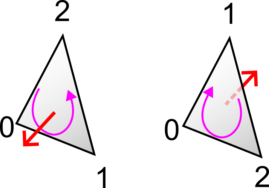
Note: the order of the indices in each face defines the face’s orientation. By convention (called the right-hand rule or counterclockwise convention), when viewing the face from outside the object, the vertices appear in counterclockwise order. This orientation enables the computation of the outward normal of the face by a cross product: \(n = (p_{i_2} - p_{i_1}) \times (p_{i_3} - p_{i_1})\). The GPU uses this information for the back-face culling: triangles viewed from behind (whose normal is oriented opposite to the camera) are not rendered, which reduces the rendering cost by about half. This convention is illustrated below.
The OBJ format (Wavefront) is one of the most widespread text formats for storing 3D meshes. Its simplicity makes it easy to read and write, as well by humans as by programs. An OBJ file is a text file where each line begins with a keyword followed by values:
v x y z: defines a vertex with its 3D
coordinates.vt u v: defines texture coordinates
(for mapping a texture onto the surface).vn x y z: defines a vertex normal
(direction perpendicular to the surface, used for shading).f v1 v2 v3: defines a triangular face
by the indices of its vertices. The indices start at 1
(and not 0). One can also reference normals and textures with the syntax
f v1/vt1/vn1 v2/vt2/vn2 v3/vt3/vn3.Minimal example (tetrahedron):```
v 0.0 0.0 0.0
v 1.0 0.0 0.0
v 0.0 1.0 0.0
v 0.0 0.0 1.0
f 1 2 4
f 1 4 3
f 1 3 2
f 2 3 4Affine transformations are the fundamental operations for positioning, orienting, and scaling objects in 3D space. In computer graphics, they are used continuously: to place an object in the scene, to animate a character (joint rotations), to position the camera, etc.
The translation moves a point by a constant vector \((t_x, t_y, t_z)\):
\[ t(p) = (x + t_x, \; y + t_y, \; z + t_z) \] Translation is not a linear transformation (it cannot be represented by multiplication by a matrix \(3 \times 3\), since \(t(0) \neq 0\) in general). This property gives rise to the need for homogeneous coordinates described later.
Scaling multiplies each coordinate by a scale factor:
\[ s(p) = (s_x \, x, \; s_y \, y, \; s_z \, z) \] In matrix notation :
\[ S = \begin{pmatrix} s_x & 0 & 0 \\ 0 & s_y & 0 \\ 0 & 0 & s_z \end{pmatrix} \] If \(s_x = s_y = s_z\), the scaling is uniform (the object preserves its proportions). Otherwise, it is non-uniform (the object is deformed, for example stretched along an axis).
A rotation preserves distances and angles (it is an isometry). It is described by an orthogonal \(3 \times 3\) matrix:
\[ R = \begin{pmatrix} a & b & c \\ d & e & f \\ g & h & j \end{pmatrix}, \quad R\,R^T = I \text{ et } \det(R) = 1 \] The columns (and rows) of \(R\) form an orthonormal basis: they are mutually orthogonal and of unit length. The condition \(\det(R) = 1\) distinguishes rotations from reflections (which have a determinant of \(-1\)).
There are several ways to parameterize a rotation in 3D: Euler angles (three successive angles around the axes), axis-angle (an axis and a rotation angle around that axis), or quaternions (a four-component representation, widely used in animation for its efficiency and absence of singularities).
Shearing shifts a coordinate in proportion to another. For example:
\[ sh_{xy}(p) = (x + \lambda \, y, \; y, \; z) \] In matrix notation :
\[ Sh_{xy} = \begin{pmatrix} 1 & \lambda & 0 \\ 0 & 1 & 0 \\ 0 & 0 & 1 \end{pmatrix} \] Shearing preserves volumes (\(\det(Sh) = 1\)) but does not preserve angles (it is not an isometry). It is rarely used intentionally in computer graphics, but may appear as a by-product of certain matrix decompositions. Its geometric effect is visible in the following figure.

Rotation and scaling are linear transformations, representable by \(3 \times 3\) matrices. Translation, however, is a non-linear transformation that cannot be encoded directly by a \(3 \times 3\) matrix.
This poses a practical problem: in computer graphics, one continually chains rotations, scalings and translations to position objects in the scene. For example, to place an object in the world frame, one can apply a scaling (to adjust its size), then a rotation (to orient it), then a translation (to position it).
If only rotations and scalings were matrices, one would need to maintain two separate representations (one matrix for the linear part and a vector for the translation), which would considerably complicate the code.
Idea: add an extra coordinate to obtain a 4D unified representation, in which all affine transformations (including translation) are expressed as matrix products.
The unified affine transformation is then written as a matrix product \(4 \times 4\) :
\[ \begin{pmatrix} p' \\ 1 \end{pmatrix} = \begin{pmatrix} L & t \\ 0 & 1 \end{pmatrix} \begin{pmatrix} p \\ 1 \end{pmatrix} = \begin{pmatrix} L\,p + t \\ 1 \end{pmatrix} \] with \(L\) the linear part (3 × 3) and \(t\) the translation vector.
For a point \(p = (x, y)\), we add a coordinate: \(p = (x, y, 1)\).
Translation becomes a linear operation :
\[ \begin{pmatrix} x + t_x \\ y + t_y \\ 1 \end{pmatrix} = \begin{pmatrix} 1 & 0 & t_x \\ 0 & 1 & t_y \\ 0 & 0 & 1 \end{pmatrix} \begin{pmatrix} x \\ y \\ 1 \end{pmatrix} \] The same applies to rotations and scaling, which are expressed as matrices \(3 \times 3\) in 2D homogeneous coordinates.
In 3D, we use four-component vectors and matrices \(4 \times 4\).
Any sequence of translations, rotations and scalings can be factorized into a unique product of matrices:
\[ M = T_0 \, R_0 \, S_0 \, T_1 \, R_1 \, S_1 \, \dots \] The advantage is substantial: regardless of the complexity of the transformation chain, the result is always a single matrix \(4 \times 4\). Applying this transformation to a point amounts to a single matrix-vector multiplication. This property is massively exploited by the GPU, which can transform millions of vertices by applying the same matrix \(M\) to each of them in parallel.
[Attention]: the order of multiplications is important. Matrix transformations are not commutative in general: \(T \, R \neq R \, T\). By convention, the transformation on the far right is applied first. Thus, \(M = T \, R \, S\) means: first scaling, then rotation, then translation.
The advantage of generalized coordinates is the natural differentiation between points and vectors :
Point : \((x, y, z, \mathbf{1})\) — the translation is applied.
\[ M \begin{pmatrix} p \\ 1 \end{pmatrix} = \begin{pmatrix} L & t \\ 0 & 1 \end{pmatrix} \begin{pmatrix} p \\ 1 \end{pmatrix} = \begin{pmatrix} L\,p + t \\ 1 \end{pmatrix} \] Vector : \((x, y, z, \mathbf{0})\) — the translation does not apply.
\[ M \begin{pmatrix} v \\ 0 \end{pmatrix} = \begin{pmatrix} L & t \\ 0 & 1 \end{pmatrix} \begin{pmatrix} v \\ 0 \end{pmatrix} = \begin{pmatrix} L\,v \\ 0 \end{pmatrix} \] This behavior is consistent with geometric operations:
This distinction is summarized in the diagram below.

Let us consider the case of a generalized point with coordinate \(w \neq 1\): \(p_{4D} = (x, y, z, w)\).
The “renormalization” (or projection) onto the space of 3D points gives: \(p_{3D} = (x/w, y/w, z/w, 1)\).
Example :
The sum of two points yields:
\[ (x_1, y_1, z_1, 1) + (x_2, y_2, z_2, 1) = (x_1+x_2, \; y_1+y_2, \; z_1+z_2, \; 2) \] After homogenization :
\[ p_{3D} = \left(\frac{x_1+x_2}{2}, \; \frac{y_1+y_2}{2}, \; \frac{z_1+z_2}{2}, \; 1\right) \] What corresponds to the barycenter of the two points.
The advantage of projective space is to encode rational operations (such as perspective) via a simple matrix multiplication.
Perspective is modeled by division by depth.
In 2D (1D projection), for a point \((x, y)\) projected onto a focal plane at distance \(f\):
\[ y' = f \, \frac{y}{x} \] This nonlinear model is written linearly in homogeneous coordinates:
\[ \begin{pmatrix} f \, y \\ x \end{pmatrix} = \begin{pmatrix} 0 & f \\ 1 & 0 \end{pmatrix} \begin{pmatrix} x \\ y \end{pmatrix} \] After homogenization (division by the last component \(x\)), we indeed obtain \(y' = f\,y/x\).
The real points (2D or 3D) are those whose last component has the value \(w = 1\) (obtained after homogenization). The vectors correspond to \(w = 0\). This projection mechanism is represented in the following figure.

A computer has two main processors for computation:
The figures below show the physical aspect and the internal architecture of these two types of processors.
CPU (gauche) et GPU (droite).
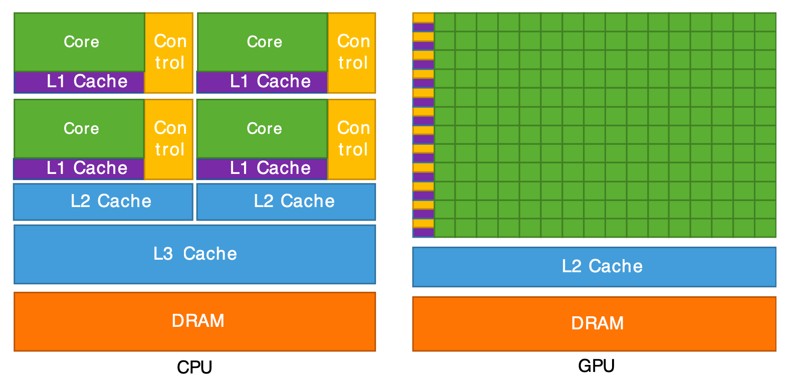
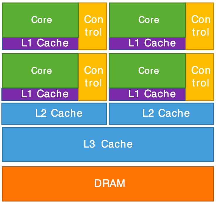
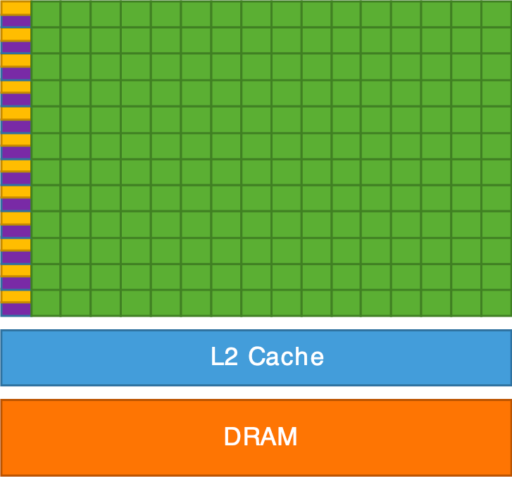
Architecture interne d'un CPU (gauche) et d'un GPU (droite).
The GPU is, in summary, a supercomputer optimized to perform the same operation on a large amount of data in parallel. That’s exactly what we need for graphics rendering: to transform millions of vertices (vertex shader) and then color millions of pixels (fragment shader). The CPU, for its part, handles the program logic (scene management, data loading, user interactions) and sends the rendering commands to the GPU.
OpenGL (Open Graphics Library) is an API (Application Programming Interface) for communicating with the GPU, oriented toward 3D graphics.
Features:
Other graphics APIs: Vulkan, WebGL, WebGPU, DirectX (Windows), Metal (Mac).
The CPU and the GPU each have their own memory (RAM and VRAM respectively) and cannot directly access each other’s memory. The rendering process therefore requires explicit communication between the two, orchestrated by the OpenGL API. This process follows three main stages:
Data preparation (CPU): the C++ program (running on the CPU) loads or computes the geometric data of the scene: vertex positions, colors, normals, texture coordinates, connectivity indices, etc. These data are organized into RAM arrays.
Sending data (CPU \(\rightarrow\) GPU): the data are transferred in blocks from RAM to VRAM via OpenGL calls. This transfer is relatively costly (the bus between CPU and GPU has limited bandwidth), which is why we aim to minimize it: ideally, static data (meshes that do not change) are sent only once at startup. Only the data that change per frame (transformation matrices, animation parameters) are transmitted per frame.
Shader Execution (GPU): once the data are in VRAM, the GPU executes shader programs in parallel on each vertex and then on each pixel. The CPU no longer intervenes during this phase: it simply issues the “draw” command and the GPU handles the rest autonomously. The result is the final image, stored in the framebuffer of VRAM, which is then displayed on the screen.
The following diagrams detail this communication pipeline.


The shaders are small programs that run directly on the GPU. They are written in a dedicated language called GLSL (OpenGL Shading Language), whose syntax is close to C. The term “shader” comes from “shading” (shading), because their initial role was to compute the shading of surfaces, but they are today used for all kinds of graphical calculations.
The fundamental peculiarity of shaders is that they are executed massively in parallel: the same program is launched simultaneously on thousands of vertices or pixels. The programmer writes the code for a single vertex or pixel, and the GPU takes care of executing it for all.
Two main types of shaders are involved in the rendering pipeline:
Executed once for each vertex of the mesh. Its main role is to transform the position of the vertex from the 3D space of the scene to the 2D space of the screen (by applying the transformation and projection matrices). It can also calculate and transmit attributes (colors, transformed normals, texture coordinates, etc.) that will be used by the fragment shader.
#version 330 core

layout(location = 0) in vec4 position;
layout(location = 1) in vec4 color;

out vec4 vertexColor;

void main()
{
    gl_Position = position;
    vertexColor = color;
}
In this example :
#version 330 core : indicates the GLSL version used
(corresponding to OpenGL 3.3).layout(location = 0) in vec4 position : declares an
input attribute (the vertex position), received from data sent by the
CPU. The location = 0 indicates the index of the attribute
buffer.out vec4 vertexColor : declares an output variable that
will be passed to the fragment shader. Between the vertex shader and the
fragment shader, this variable will be automatically interpolated by
rasterization.gl_Position : a predefined special variable provided by
OpenGL, in which the vertex shader must write the final position of the
vertex (in clip coordinates).Executed once for each pixel (fragment) covered by a triangle after rasterization. Its role is to determine the final color of the pixel based on the interpolated attributes (color, normal, texture coordinates), lighting, textures, etc. It is in the fragment shader that we implement illumination models and visual effects.
#version 330 core

in vec4 vertexColor;
out vec4 fragColor;

void main()
{
    fragColor = vertexColor;
}
In this example:
in vec4 vertexColor : input variable coming from the
vertex shader. Its value has been automatically interpolated by
rasterization between the three vertices of the current triangle, using
the fragment’s barycentric coordinates.out vec4 fragColor : the output color of the fragment,
which will be written to the final image (framebuffer).In addition to attributes (per-vertex) and interpolated variables (per-fragment), shaders can receive uniform variables (uniform): constant values for all vertices or fragments in a single render call. They are defined on the CPU side and sent to the GPU. Typical examples are transformation matrices, the camera position, the light direction, the current time, etc.
uniform mat4 modelViewProjection; // matrice de transformation (4x4)
uniform vec3 lightDirection;      // direction de la lumière
The full pipeline works as follows:
The attributes transmitted from the vertex shader to the fragment
shader (such as vertexColor) are automatically
interpolated barycentrically between the triangle’s
vertices, which exactly corresponds to the barycentric interpolation
described above. The entirety of this pipeline is summarized in the
diagram below.

As seen in the previous chapter, a 3D scene is described by models (surfaces), light sources, and a camera. Rendering by rasterization yields a 2D image of this scene.
However, at the level of the GPU and OpenGL, there is no explicit notion of a camera or light. The GPU manipulates only vertices with their attributes (position, color, normal, etc.) as input to the vertex shader, and fragments (pixels) colored as output of the fragment shader. The programmer’s job is to translate high-level concepts (camera, light, materials) into operations on the vertices and fragments via shaders.
The rendering pipeline breaks down into three main stages. The first is the transformation of the vertices, performed by the vertex shader: each vertex is projected from the 3D space of the scene to the 2D space of the screen by applying the transformation and projection matrices. The second stage is the rasterization: the triangles projected in 2D are converted into fragments (pixels) by an automatic discretization process. Finally, the third stage is the color calculation, performed by the fragment shader: for each fragment, its final color is determined based on lighting, the material and the textures.
OpenGL only draws triangles whose vertices lie inside the cube \([-1, 1]^3\). This normalized space is called Normalized Device Coordinates (NDC). The first two components \((x_{\text{ndc}}, y_{\text{ndc}})\) correspond to the screen coordinates, whereas \(z_{\text{ndc}}\) encodes the depth, i.e., the distance to the camera in image space. This normalized cube is depicted in the following figure.

The goal of projection is to convert the global coordinates (world space) to NDC coordinates. This conversion must, on the one hand, define a camera model that specifies which part of 3D space is visible, and on the other hand apply the perspective so that distant objects appear smaller than nearby objects.
The most common perspective model uses a viewing volume in the shape of a pyramid frustum (frustum), delimited by a near plane (\(z_{\text{near}}\)) and a far plane (\(z_{\text{far}}\)), as illustrated below.

Let a point with coordinates \((x, y, z)\) in world space. The NDC coordinates \((x_{\text{ndc}}, y_{\text{ndc}}, z_{\text{ndc}})\) are computed as follows:
Coordinates \(x\) and \(y\):
\[ x_{\text{ndc}} = \frac{z_{\text{near}}}{-z} \cdot \frac{x}{w} = \frac{1}{\tan(\theta/2)} \cdot \frac{x}{-z} \]
\[ y_{\text{ndc}} = \frac{z_{\text{near}}}{-z} \cdot \frac{y}{h} = \frac{r}{\tan(\theta/2)} \cdot \frac{y}{-z} \] where \(\theta\) is the field of view (Field of View, FOV) and \(r = h/w\) is the aspect ratio.
Division by \(-z\) produces the perspective effect: distant objects (large \(|z|\)) are reduced in size.
Z coordinate \(z\) (depth) :
The NDC depth is a non-linear function of \(z\) :
\[ z_{\text{ndc}} = \frac{1}{-z} \left( -\frac{z_{\text{far}} + z_{\text{near}}}{z_{\text{far}} - z_{\text{near}}} \cdot z - \frac{2 \, z_{\text{near}} \, z_{\text{far}}}{z_{\text{far}} - z_{\text{near}}} \right) \] with the correspondences: \(z = -z_{\text{near}} \rightarrow z_{\text{ndc}} = -1\) and \(z = -z_{\text{far}} \rightarrow z_{\text{ndc}} = 1\).
The variation in \(1/z\) implies a finer precision near the camera and coarser as the distance increases. This is a deliberate choice: nearby objects require better depth resolution to avoid visual artifacts.
In homogeneous coordinates, the projection is expressed as a \(4 \times 4\) matrix product:
\[ p_{\text{ndc}} = \text{Proj} \times p \] with :
\[ \text{Proj} = \begin{pmatrix} \frac{1}{\tan(\theta/2)} & 0 & 0 & 0 \\ 0 & \frac{r}{\tan(\theta/2)} & 0 & 0 \\ 0 & 0 & -\frac{z_{\text{far}} + z_{\text{near}}}{z_{\text{far}} - z_{\text{near}}} & -\frac{2 \, z_{\text{near}} \, z_{\text{far}}}{z_{\text{far}} - z_{\text{near}}} \\ 0 & 0 & -1 & 0 \end{pmatrix} \] After multiplication, the obtained vector has a component \(w \neq 1\). The homogenization (division by \(w\)) produces the final NDC coordinates. This is exactly the mechanism of projective space seen in the previous chapter.
The result is a deformed space inside the cube \([-1, 1]^3\). The final image corresponds to the view \((x_{\text{ndc}}, y_{\text{ndc}})\) of this cube, while \(z_{\text{ndc}}\) represents the depth seen from the camera in image space. Everything outside the cube \([-1, 1]^3\) is automatically discarded by the GPU (clipping).
The variation in \(1/z\) of the NDC depth has an important consequence: the precision depends strongly on the choice of \(z_{\text{near}}\). The following diagram shows this nonuniform distribution of precision.

If \(z_{\text{near}}\) is too close to 0, all precision is concentrated on distances very close to the camera. Distant objects end up with depth values almost identical after discretization. This causes a visual artifact called z-fighting (or depth-fighting): two surfaces close in depth “flicker” randomly because the GPU cannot determine which is in front. The graph below illustrates the curve of \(z_{\text{ndc}}\) as a function of \(z\).
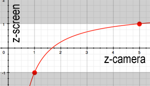
Practical rule: choose \(z_{\text{near}}\) as large as possible (while keeping objects visible in the frustum) to maximize depth precision across the entire scene.
The view matrix transforms coordinates from world space to camera space (view space). It positions and orients the camera in the scene, according to the principle illustrated below.

The camera is described by a \(4 \times 4\) matrix containing its local axes and its position:
\[ \text{Cam} = \begin{pmatrix} \text{right}_x & \text{up}_x & \text{back}_x & \text{eye}_x \\ \text{right}_y & \text{up}_y & \text{back}_y & \text{eye}_y \\ \text{right}_z & \text{up}_z & \text{back}_z & \text{eye}_z \\ 0 & 0 & 0 & 1 \end{pmatrix} = \begin{pmatrix} O & \text{eye} \\ 0 & 1 \end{pmatrix} \] where \(O = (\text{right}, \text{up}, \text{back})\) is the camera rotation matrix (orthonormal basis) and \(\text{eye}\) is its position in the world.
The view matrix is the inverse of the camera matrix:
\[ \text{View} = \text{Cam}^{-1} = \begin{pmatrix} O^T & -O^T \cdot \text{eye} \\ 0 & 1 \end{pmatrix} \] This inversion is very efficient to compute because \(O\) is orthogonal (\(O^{-1} = O^T\)). The view matrix maps the camera position to the origin and aligns its axes with the axes of the frame.
The model matrix positions an object in the world. It transforms the object’s local coordinates to the world space coordinates:
\[ \text{Model} = \begin{pmatrix} R & t \\ 0 & 1 \end{pmatrix} \] where \(R\) is the rotation matrix (orientation of the object) and \(t\) is the translation vector (position of the object). The following figure shows this passage from local coordinates to world space.

The importance of separating an object’s geometry from its position is fundamental. The object’s geometric coordinates (mesh) are loaded only once into VRAM, and to move or orient the object, it suffices to modify the Model matrix, namely a simple matrix \(4 \times 4\) of 16 floats. This separation also enables instancing: the same mesh can be drawn at several locations in the scene by applying different Model matrices, without duplicating the geometric data in memory. For example, a forest consisting of thousands of trees may store only a single tree mesh, each instance having its own Model matrix (position, rotation, scale).
The complete transformation of a vertex, from its local coordinates to NDC space, is the composition of the three matrices:
\[ p_{\text{ndc}} = \text{Proj} \times \text{View} \times \text{Model} \times p \] The vertex starts from its local coordinates \(p = (x, y, z, 1)\) in the object space, where the geometry is defined relative to the object’s origin. The Model matrix places it in the world space: \(p_{\text{world}} = \text{Model} \times p\), applying the object’s rotation, scale, and translation. The View matrix then transforms this position into the camera space: \(p_{\text{view}} = \text{View} \times p_{\text{world}}\), where the camera is at the origin and looks in the direction \(-z\). Finally, the Projection matrix converts the coordinates to NDC: \(p_{\text{ndc}} = \text{Proj} \times p_{\text{view}}\), applying perspective and normalizing the coordinates into the cube \([-1, 1]^3\) after homogenization (division by \(w\)).
This chain constitutes the first stage of the graphics pipeline, performed by the vertex shader.
#version 330 core

layout (location = 0) in vec3 vertex_position;

uniform mat4 model;
uniform mat4 view;
uniform mat4 projection;

void main() {
    gl_Position = projection * view * model * vec4(vertex_position, 1.0);
}
The three matrices are sent to the GPU as uniform variables from the C++ code. The GPU then applies this transformation in parallel on all vertices. This is much more efficient than computing the new positions on the CPU: instead of transferring \(N\) modified positions per frame, we transfer only three matrices \(4 \times 4\) (i.e., 48 floats).
void main_loop() {
    // Mise à jour des matrices
    glUniform(shader, Model);
    glUniform(shader, View);
    glUniform(shader, Projection);

    draw(mesh_drawable);
}The rasterization (or rasterisation, or facetization) is the conversion of vector data (triangles defined by vertices) into discrete elements: des? Wait—this must be translated consistently.
The conversion of vector data (triangles defined by vertices) into discrete elements: pixels (or fragments). It is an automatic and non-programmable step in the OpenGL pipeline.
The fundamental operation is the following: given a triangle defined by three 2D points (after projection), determine the set of pixels it covers, as can be seen in the following figure.

Before tackling the rasterization of triangles, consider simpler primitives to understand the principle of discretization.
Point : a single pixel.
im(x0, y0) = c;Rectangle : two nested loops.
for(int kx = x0; kx < x1; kx++)
    for(int ky = y0; ky < y1; ky++)
        im(kx, ky) = c;
Horizontal, vertical or diagonal segment: a single loop suffices.
// Segment horizontal
for(int kx = x0; kx < x1; kx++)
    im(kx, y0) = c;
For an arbitrary segment, the discretization is no longer trivial: several pixelated approximations are possible, as shown in the image below. One must choose an efficient and deterministic algorithm.
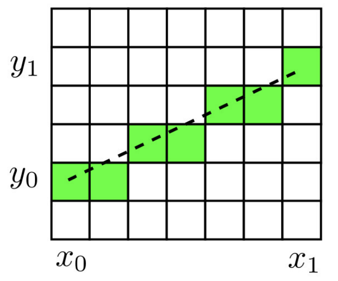
The Bresenham’s algorithm is a classic and very efficient algorithm for rasterizing a segment. It relies solely on integer operations, which makes it fast and accurate.
Principle: we move along the x-axis pixel by pixel. At each step, we evaluate whether the accumulated error in \(y\) exceeds \(0.5\) :
The progression of the algorithm is visualized in the following figure.

int dx = x1 - x0, dy = y1 - y0;
float a = float(dy) / float(dx);
float erreur = 0.0f;

int y = y0;
for(int x = x0; x <= x1; x++)
{
    im(x, y) = c;
    erreur += a;
    if(erreur >= 0.5f)
    {
        y = y + 1;
        erreur = erreur - 1.0f;
    }
}
Note: by multiplying all values by \(2 \, dx\), one can eliminate divisions and floating-point operations to obtain a purely integer algorithm. The algorithm above handles the case \(0 \leq dy \leq dx\); the other octants are treated by symmetry.
The rasterization of a triangle \((p_0, p_1, p_2)\) is performed by the scanline algorithm:
Discretize the edges: for each edge of the triangle (\((p_0, p_1)\), \((p_1, p_2)\), \((p_2, p_0)\)), apply the Bresenham algorithm to obtain the boundary pixels.
Store the horizontal bounds: for each line \(y\), store the values \(x_{\min}\) and \(x_{\max}\) of the boundary pixels.
Fill line by line: for each line \(y\), color all the pixels from \(x_{\min}\) to \(x_{\max}\).
The two steps are illustrated below: edge discretization and filling.


Rasterization d'un triangle par scanline : discrétisation des arêtes (gauche) et remplissage horizontal (droite).
Example of a scanline table for a triangle :
| \(y\) | \(x_{\min}\) | \(x_{\max}\) |
|---|---|---|
| 0 | 3 | 5 |
| 1 | 0 | 5 |
| 2 | 1 | 4 |
| 3 | 2 | 4 |
| 4 | 3 | 3 |
During rasterization, the barycentric coordinates of each fragment are computed to interpolate the vertex attributes (color, normal, texture coordinates, depth) linearly inside the triangle.
The Phong model is the most classic illumination model in real-time rendering. It rests on the observation that the appearance of a lit surface can be decomposed into three distinct physical phenomena. The first is the ambient component, which represents a uniform base color, independent of geometry and light position: it roughly models the indirect light that bathes the entire scene. The second is the diffuse component, which depends on the local orientation of the surface relative to the light: a surface facing the light is bright, a surface facing the other way is dark. The third is the specular component, which models the shiny reflection of the light source visible on smooth surfaces, and which depends on the observer’s viewpoint. These three contributions are represented on the following figure.

The final color of a point is the sum of these three components:
\[ C = C_a + C_d + C_s \] The calculation of each component involves two color properties: the color of the light source \(C_\ell = (r_\ell, g_\ell, b_\ell) \in [0, 1]^3\) and the color of the surface (or albedo) \(C_o = (r_o, g_o, b_o) \in [0, 1]^3\). Their component-wise multiplication (\((r_\ell \cdot r_o, \, g_\ell \cdot g_o, \, b_\ell \cdot b_o)\)) models the filtering of light by the material: a red surface illuminated by white light appears red, while the same surface illuminated by a green light appears black (because the red component of the light is zero).
The ambient component models a uniform illumination of the scene (approximate indirect lighting). It does not depend on either the position or the orientation of the surface:
\[ C_a = \alpha_a \, C_\ell \, C_o \] with \(\alpha_a \in [0, 1]\) the ambient coefficient. This term prevents surfaces that are not directly illuminated from being completely black.
The diffuse component models the light reflected uniformly in all directions by a matte surface (Lambertian reflection). It depends on the angle between the normal \(n\) to the surface and the direction of the light \(u_\ell\):
\[ C_d = \alpha_d \, (n \cdot u_\ell)_+ \, C_\ell \, C_o \] The coefficient \(\alpha_d \in [0, 1]\) controls the diffuse reflection intensity of the material. The central term is the diffuse factor \((n \cdot u_\ell)_+ = \max(n \cdot u_\ell, \, 0)\), which is the dot product between the unit normal vector \(n\) to the surface and the unit direction \(u_\ell\) from the point toward the light source. This dot product measures the cosine of the angle between the normal and the direction of the light. When the surface faces the light directly (\(n\) parallel to \(u_\ell\)), the factor equals 1 and the illumination is maximal. When the surface is grazing (\(n\) perpendicular to \(u_\ell\)), the factor equals 0. When the surface is turned opposite to the light, the dot product is negative, and the truncation \(\max(\cdot, 0)\) forces the contribution to zero, avoiding physically absurd lighting.
This geometric mechanism is schematically illustrated below.

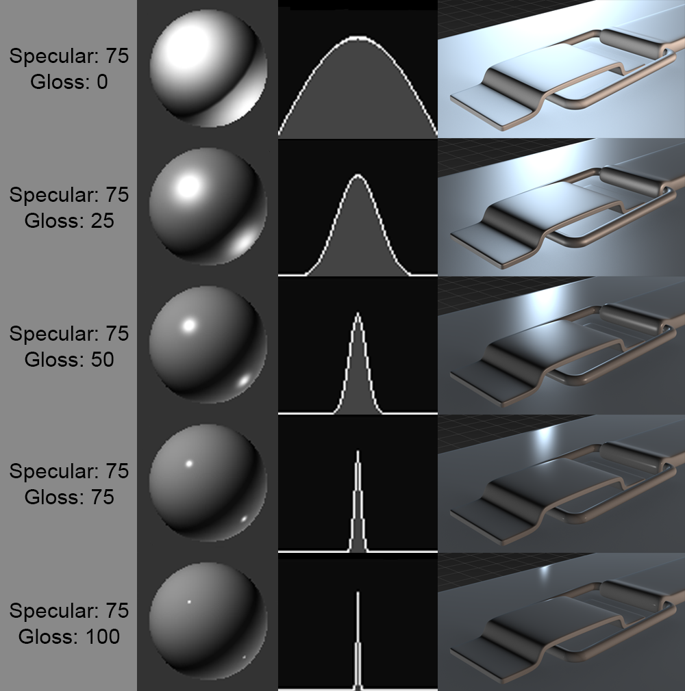
The specular component models the reflection of the light source on the surface. Unlike the diffuse component, it depends on the camera’s viewpoint:
\[ C_s = \alpha_s \, (u_r \cdot u_v)_+^{s_{\exp}} \, C_\ell \] The coefficient \(\alpha_s \in [0, 1]\) controls the intensity of the specular reflection. The shininess exponent \(s_{\exp}\) (typically between 64 and 256) determines the size of the highlight: the higher it is, the more the highlight is concentrated in a narrow and sharp spot (very polished surface), while a low exponent produces a broad and diffuse highlight (slightly rough surface).
The vector \(u_r\) is the
direction of reflection of the light with respect to
the normal, calculated by the formula \(u_r =
2 \, (u_\ell \cdot n) \, n - u_\ell\) (in GLSL:
reflect(-u_l, n)). The vector \(u_v\) is the unit direction from the
surface point toward the camera. The dot product \((u_r \cdot u_v)\) measures the alignment
between the reflection direction and the viewing direction: the
highlight is maximal when the observer lies exactly in the mirror
reflection direction of the light.
The specular component does not depend on the color of the surface \(C_o\) but only on \(C_\ell\), which corresponds to the physical behavior of reflections on dielectric materials (plastic, ceramic, etc.) : the reflection of white light on a red surface remains white. The geometry of the specular reflection and the influence of the shininess exponent are detailed in the following figures.

The Phong model defines the illumination formula at a point on the surface, but the question remains where and how often this formula is evaluated. Three classic strategies exist, with a trade-off between computational cost and visual quality.
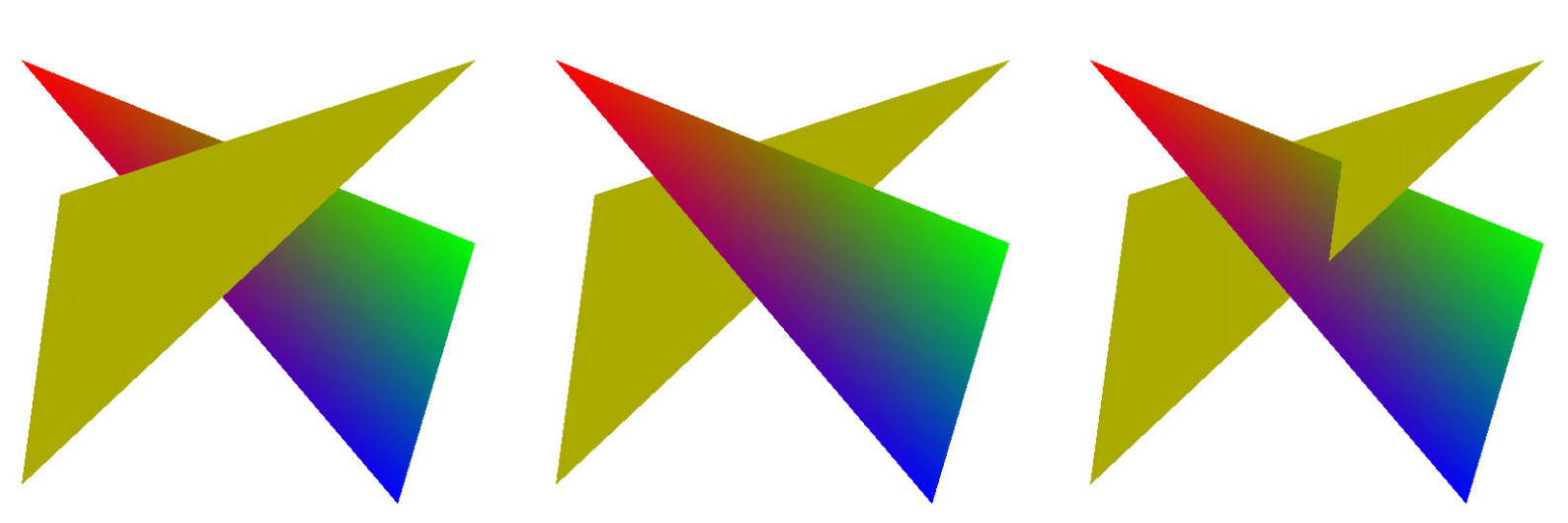
The flat shading is the simplest approach: the color is computed once per triangle, using the geometric normal of the face. All pixels of the triangle receive exactly the same color. The result has a faceted appearance where every triangle is clearly visible, which may be acceptable for non-photorealistic rendering but is unsuitable for smooth surfaces.
The Gouraud shading improves quality by computing the illumination at the vertices of the triangle (in the vertex shader), then by linearly interpolating the resulting color inside the triangle during rasterization. The color transitions between adjacent triangles become smooth, giving the appearance of a smooth surface. However, this approach presents an important drawback: if a specular highlight falls in the middle of a large triangle, far from any vertex, it will be completely missed because no vertex has “seen” the reflection.
The Phong shading solves this problem by interpolating not the color, but the normal between the triangle’s vertices. The illumination is then calculated for each fragment (in the fragment shader) with this interpolated normal. The specular reflection is thus correctly computed at every point on the surface, even at the center of a large triangle. The visual difference among these three approaches is shown in the following figure.
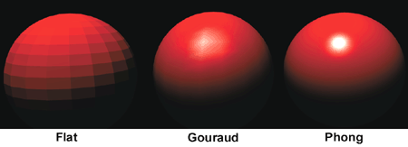
In practice, the Phong shading is the standard. The overhead relative to Gouraud shading is negligible on modern GPUs (the fragment shader performs a few additional operations per pixel, but the GPU has thousands of cores to execute them in parallel), and the visual quality is significantly higher.
The Phong model naturally extends to multiple light sources by summing the contributions of each light:
\[ C = \sum_i \left( \alpha_a \, C_{\ell_i} \, C_o + \alpha_d \, (n \cdot u_{\ell_i})_+ \, C_{\ell_i} \, C_o + \alpha_s \, (u_{r_i} \cdot u_v)_+^{s_{\exp}} \, C_{\ell_i} \right) \] #### Distance attenuation
In physical reality, the light intensity of a point light source decreases proportionally to the inverse square of the distance (\(1/r^2\)). In real-time rendering, one often uses a simplified attenuation model that decreases linearly up to a maximum distance, beyond which the light has no effect:
\[ C_\ell(p) = \left(1 - \min\left(\frac{\|p - p_\ell\|}{d_{\text{att}}}, \, 1\right)\right) \, C_\ell^0 \] The vector \(p\) is the position of the point on the surface, \(p_\ell\) the position of the light, \(d_{\text{att}}\) the characteristic attenuation distance (beyond which the contribution is zero), and \(C_\ell^0\) the color of the light at the source. This linear model is less realistic than the \(1/r^2\) law, but it has the advantage of guaranteeing that the light dies out completely beyond \(d_{\text{att}}\), which allows rendering to be optimized by ignoring lights that are too far away.
An atmospheric fog effect simulates the absorption and scattering of light by the atmosphere. The principle is to progressively blend the calculated color with a uniform fog color as a function of the distance to the camera:
\[ C_{\text{final}} = (1 - \gamma(p)) \, C + \gamma(p) \, C_{\text{fog}} \] The fog blending factor \(\gamma(p) = \min( \|p - p_{\text{eye}}\| / d_{\text{fog}}, 1 )\) varies from 0 (near object, color unchanged) to 1 (far object, completely immersed in fog). The parameter \(d_{\text{fog}}\) controls the distance at which the fog becomes completely opaque, and \(C_{\text{fog}}\) is the color of the fog (often a light gray or the color of the sky). In practice, this effect provides a sense of atmospheric depth and naturally masks the far clipping plane (\(z_{\text{far}}\)), avoiding the abrupt disappearance of objects at the horizon.
The toon shading (or cel shading) is a non-photorealistic effect that gives a cartoon-like appearance. The principle is to discretize the color values into steps:
\[ C_{\text{toon}} = \frac{\text{floor}(C \times N)}{N} \] where \(N\) is the number of desired levels. This subsampling creates discrete color bands characteristic of the cartoon style, of which an example is shown below.
When several triangles overlap on the screen, it is necessary to determine which one is visible for each pixel. Without an occlusion mechanism, the order in which the triangles are rendered determines the result, which is incorrect, as demonstrated by the following image.
The Z-buffer (or depth buffer) is an auxiliary image of the same resolution as the final image, which stores the depth value \(z_{\text{ndc}}\) of the fragment closest to the camera for each pixel.
The algorithm is simple: for each fragment to be drawn, we compare its depth with the value stored in the Z-buffer:
def draw(position, couleur, z, image, zbuffer):
    if z < zbuffer(position):
        image(position) = couleur
        zbuffer(position) = z
    # sinon: ne rien dessiner (fragment masqué)
The contents of the Z-buffer can be visualized as a grayscale image.
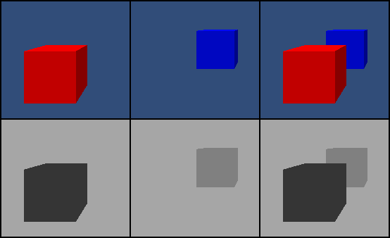
The Z-buffer is initialized to the maximum depth value (1.0, corresponding to the far plane) at the start of every frame. Each fragment updates the Z-buffer if its depth is smaller (closer to the camera) than the stored value. This ensures that only the closest fragment is drawn, independently of the drawing order of the triangles.
This step is performed automatically by the GPU (not programmable),
provided that depth testing is enabled
(glEnable(GL_DEPTH_TEST) in OpenGL).
The complete rendering pipeline chains together several steps in sequence. The vertex shader first transforms each vertex by applying the matrix chain Projection \(\times\) View \(\times\) Model, and passes the transformed attributes (world-space position, normal, color) to the next stages. The transformed vertices are then grouped into triangles during the assembly of primitives, using the connectivity table sent from the CPU.
The rasterization takes each triangle projected in 2D and determines the set of pixels it covers. For each covered pixel (called a fragment), the attributes of the triangle’s three vertices are interpolated barycentrically. The fragment shader receives these interpolated attributes and computes the final color of the fragment by applying the Phong illumination model. The depth test (Z-buffer) then compares the fragment’s depth with the value stored for that pixel: only the fragment closest to the camera is kept, the others are discarded. The result of this sequence of steps is the final image, stored in the framebuffer and displayed on the screen.
The full sequence of these steps is summarized in the diagram below.

Vertex shader : transforms the positions and normals, transmits the attributes to the fragment shader.
#version 330 core

layout (location = 0) in vec3 vertex_position;
layout (location = 1) in vec3 vertex_normal;
layout (location = 2) in vec3 vertex_color;

out struct fragment_data {
    vec3 position;
    vec3 normal;
    vec3 color;
} fragment;

uniform mat4 model;
uniform mat4 view;
uniform mat4 projection;

void main() {
    vec4 position = model * vec4(vertex_position, 1.0);

    mat4 modelNormal = transpose(inverse(model));
    vec4 normal = modelNormal * vec4(vertex_normal, 0.0);

    fragment.position = position.xyz;
    fragment.normal   = normal.xyz;
    fragment.color    = vertex_color;

    gl_Position = projection * view * position;
}
Note: the normal is transformed by the transpose of the inverse of
the Model matrix (transpose(inverse(model))), and not by
the Model matrix directly. Indeed, if the Model matrix contains a
non-uniform scaling, the direct multiplication would distort the normals
and the shading would be incorrect.
Fragment shader : calculates Phong illumination for each fragment.
#version 330 core

in struct fragment_data {
    vec3 position;
    vec3 normal;
    vec3 color;
} fragment;

uniform vec3 light_position;
uniform vec3 light_color;

layout(location = 0) out vec4 FragColor;

void main() {
    vec3 N = normalize(fragment.normal);
    vec3 L = normalize(light_position - fragment.position);

    float diffuse_magnitude = max(dot(N, L), 0.0);

    vec3 c = 0.1 * fragment.color * light_color;                    // ambiante
    c = c + 0.7 * diffuse_magnitude * fragment.color * light_color;  // diffuse
    // + composante spéculaire (omise pour simplifier)

    FragColor = vec4(c, 1.0);
}
The variables fragment.position,
fragment.normal and fragment.color are
automatically interpolated barycentrically by the GPU
between the values of the three vertices of the current triangle.
A mesh (mesh) is a set of polygons sharing vertices. It is described by :
Depending on the type of polygons used, we distinguish :
These three categories are illustrated below.
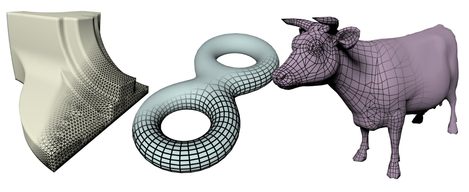
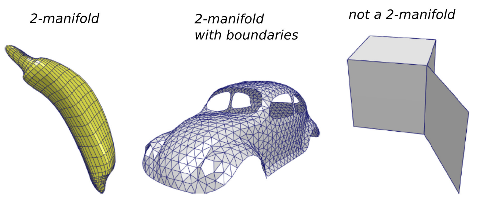
A mesh represents a manifold (manifold) if each edge is shared by at most 2 faces, as illustrated in the following figure. This property guarantees that the surface is locally equivalent to a plane (or a half-plane at the boundary), which is necessary for most mesh processing algorithms.
The standard encoding of a triangular mesh in C++ uses two arrays:
struct vec3 { float x, y, z; };
struct int3 { int i, j, k; };

std::vector<vec3> position;      // positions des sommets
std::vector<int3> connectivity;  // indices des faces (triplets)
The use of std::vector guarantees the memory
contiguity, essential for efficient transfer to the GPU.
Example: tetrahedron
std::vector<vec3> position = { {0,0,0}, {1,0,0}, {0,1,0}, {0,0,1} };
std::vector<int3> connectivity = { {0,1,2}, {0,1,3}, {0,2,3}, {1,2,3} };
Example: planar mesh
std::vector<vec3> position = { p0, p1, p2, p3, p4, p5, p6, p7, p8 };
std::vector<int3> connectivity = { {0,1,3}, {1,2,3}, {0,3,4}, {3,5,4},
                                   {2,5,3}, {2,6,5}, {5,6,7}, {5,7,8}, {4,5,8} };
The following diagram shows the correspondence between the indices and the geometry of the mesh.

Note on orientation : the triplets \((0, 1, 3)\), \((1, 3, 0)\) and \((3, 0, 1)\) are equivalent (cyclic permutation). By contrast, \((0, 1, 3)\) has an orientation inverse to \((3, 1, 0)\), \((1, 0, 3)\) or \((0, 3, 1)\). The orientation determines the direction of the normal and thus the sense of the face (see previous chapter).
The typical workflow for displaying a mesh with OpenGL follows these steps:
mesh_drawable variable
(shared between methods).mesh structure containing
the data arrays in RAM (CPU).mesh to the
mesh_drawable in VRAM (GPU).draw() which activates the shader, sends the
uniforms and launches the rendering.This flow is summarized in the diagram below.

In practice, each vertex carries additional attributes beyond its position: normals, texture coordinates, colors, etc.
std::vector<vec3> position     = { p_0, p_1, p_2, p_3 };
std::vector<vec3> normal       = { n_0, n_1, n_2, n_3 };
std::vector<vec3> color        = { c_0, c_1, c_2, c_3 };
std::vector<vec2> uv           = { uv_0, uv_1, uv_2, uv_3 };
std::vector<int3> connectivity = { {0,1,2}, {0,1,3}, {0,2,3}, {1,2,3} };
with \(p_i = (x_i, y_i, z_i)\), \(n_i = (n_{x_i}, n_{y_i}, n_{z_i})\) with \(\|n_i\| = 1\), and \(c_i = (r_i, g_i, b_i)\). The following figure represents these different attributes on a mesh.

Key points:
Sometimes, it is necessary to duplicate a vertex when it occupies the same position but with different attributes depending on the face considered. The most common case is that of sharp edges.
Consider a vertex located at a position \(p_A\) where two groups of faces meet at a right angle. If one desires a rendering with a crisp edge (not smoothed), the vertex must carry two different normals, one for each group of faces. Since the connectivity table is unique, one must create two distinct entries in the vertex array, sharing the same position but with different normals.
// Avant duplication : sommet v4 à la position pA avec une seule normale
std::vector<vec3> position = { p0, p1, p2, p3, pA, pB };
std::vector<vec3> normal   = { n0, n0, n1, n1, n2, n2 };

// Après duplication : v4 et v6 partagent pA mais avec des normales différentes
std::vector<vec3> position = { p0, p1, p2, p3, pA, pB, pA, pB };
std::vector<vec3> normal   = { n0, n0, n1, n1, n1, n1, n0, n0 };
The principle is visible in the following diagram.

For a cube, each geometric vertex is shared by 3 perpendicular faces. Since each face requires a different normal, each vertex is duplicated 3 times, i.e., \(8 \times 3 = 24\) vertices instead of 8.
A common case of meshing is the discretization of parametric surfaces.
Let a surface \(S(u, v) = (S_x(u,v), \, S_y(u,v), \, S_z(u,v))\) with \((u, v) \in [0, 1]^2\), uniformly sampled on a grid \(N_u \times N_v\), the structure of which is shown below.

The construction of the mesh is done in two steps :
Vertex positions :
for(int ku = 0; ku < Nu; ku++) {
    for(int kv = 0; kv < Nv; kv++) {
        float u = ku / (Nu - 1.0f);
        float v = kv / (Nv - 1.0f);
        S.position[kv + Nv * ku] = { Sx(u,v), Sy(u,v), Sz(u,v) };
    }
}
Connectivity (two triangles per grid cell) :
for(int ku = 0; ku < Nu - 1; ku++) {
    for(int kv = 0; kv < Nv - 1; kv++) {
        unsigned int idx = kv + Nv * ku;
        uint3 triangle_1 = { idx, idx + 1 + Nv, idx + 1 };
        uint3 triangle_2 = { idx, idx + Nv, idx + 1 + Nv };
        S.connectivity.push_back(triangle_1);
        S.connectivity.push_back(triangle_2);
    }
}
This scheme applies to many surfaces, as shown by the following examples.
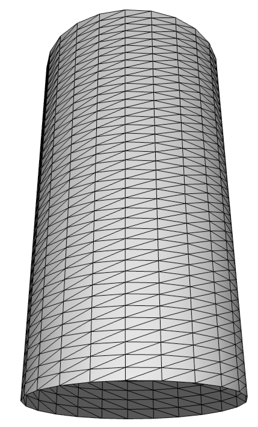
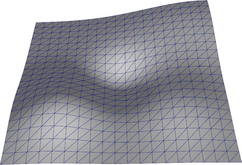
Exemples de surfaces paramétriques : cylindre (gauche) et terrain (droite).
Normals are not always provided (files without normals, procedural meshes, real-time deformations). It is then necessary to calculate from geometry.
The standard method consists in computing the unweighted average of the normals of the neighboring triangles of each vertex :
\[ n_i = \frac{\sum_{t \in \mathcal{N}_i} n_t}{\left\| \sum_{t \in \mathcal{N}_i} n_t \right\|} \] This process is illustrated below.

Implementation :
std::vector<vec3> normal(position.size(), {0,0,0});

// Accumulation par triangle
for(int t = 0; t < connectivity.size(); t++) {
    int a = connectivity[t][0];
    int b = connectivity[t][1];
    int c = connectivity[t][2];

    vec3 n = cross(position[b] - position[a], position[c] - position[a]);
    n = normalize(n);

    normal[a] += n;
    normal[b] += n;
    normal[c] += n;
}

// Normalisation finale
for(int k = 0; k < normal.size(); k++) {
    normal[k] = normalize(normal[k]);
}
If vertices are duplicated (sharp edges), the computed normals will naturally differ for each copy, since they do not share the same neighboring triangles, as can be seen in the following figure.

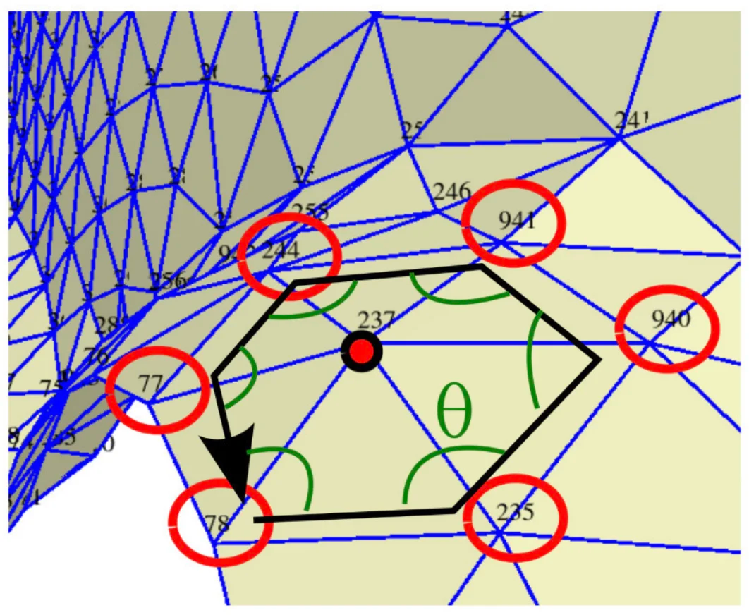
The 1-ring of a vertex is the set of triangles that share this vertex. This neighborhood structure is useful for many algorithms (normal calculation, smoothing, subdivision, etc.).
std::vector<std::vector<int>> one_ring;
one_ring.resize(position.size());
for(int k_tri = 0; k_tri < connectivity.size(); k_tri++) {
for(int k = 0; k < 3; k++) {
one_ring[connectivity[k_tri][k]].push_back(k_tri);
}
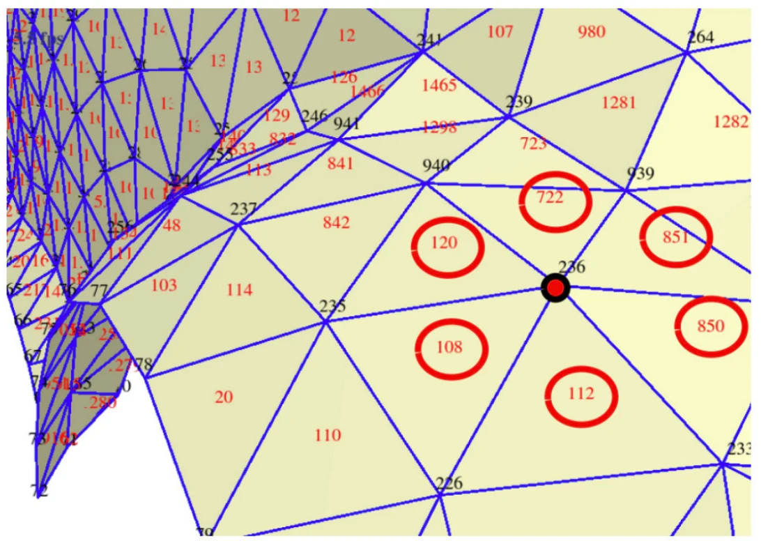
}For example:
one_ring[235] = {842, 120, 108, 110, 20, 114};
one_ring[236] = {108, 112, 851, 850, 120, 722};
The figure below illustrates this notion of neighborhood.
The half-edge (half-edge) structure is a data structure richer than the simple connectivity table. It encodes the edges in an oriented manner: each edge is represented by two half-edges with opposite directions, as shown in the diagram below. Faces appear as loops along the half-edges.
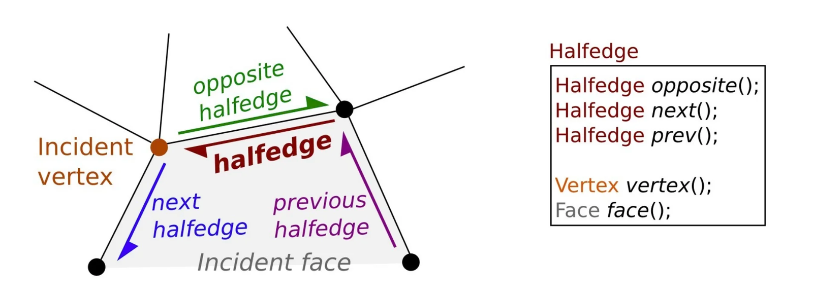
Advantages :
Limitations :
Example with CGAL :
typedef CGAL::Cartesian<double> Kernel;
typedef CGAL::Polyhedron_3<Kernel> Polyhedron;

int main() {
    Polyhedron mesh;
    std::ifstream stream("mesh.off");
    stream >> mesh;

    int face_number = 0;
    for(auto it_face = mesh.facets_begin();
        it_face != mesh.facets_end(); ++it_face)
    {
        auto halfedge = it_face->halfedge();
        auto const halfedge_end = halfedge;
        do {
            const auto p = halfedge->vertex()->point();
            std::cout << p << std::endl;
            halfedge = halfedge->next();
        } while(halfedge != halfedge_end);
        face_number++;
    }
}The objective of textures is to provide a color detail level finer than the geometry. A triangle can have a uniform color or be interpolated between its vertices, but this remains limited. Textures allow mapping a detailed 2D image onto the 3D surface.
The classic case is the UV-mapping: a 2D image (the texture) is associated with the surface 3D via texture coordinates \((u, v)\) (also denoted \((s, t)\)).
The mechanism is illustrated below.
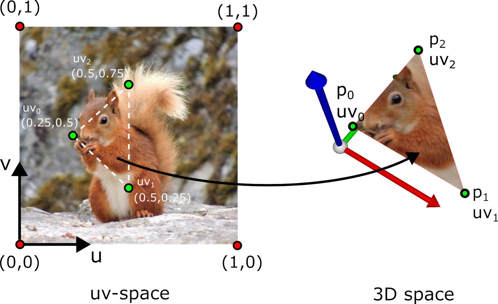
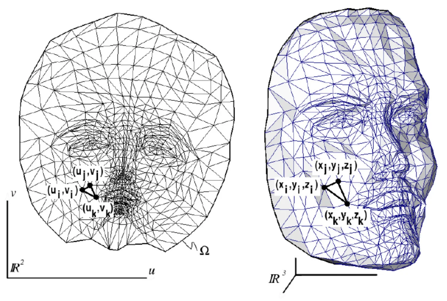
Principe de l'UV-mapping : association entre coordonnées 2D de la texture et surface 3D.
The convention is that \((0, 0)\) corresponds to the bottom-left corner of the image and \((1, 1)\) to the top-right corner.
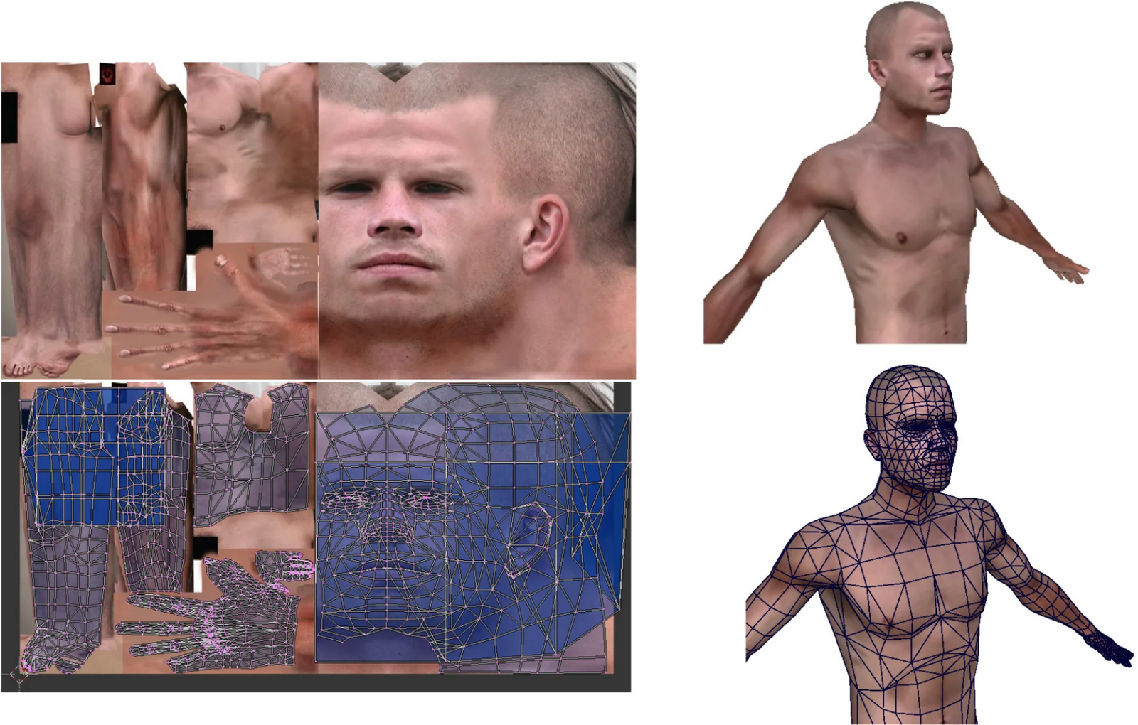
For complex models, UV unfolding is performed in pieces (patches or islands). The process comprises the following steps:
Patch cutting: the surface is cut along seams (seams) chosen by the artist or an automatic algorithm. Seams are placed in less visible areas (creases, back of the object).
Unfolding: each patch is unfolded in the 2D plane while minimizing deformations. Classical algorithms include ABF (Angle-Based Flattening), LSCM (Least Squares Conformal Maps) and Slim (Scalable Locally Injective Mappings).
Packing: the unfolded patches are arranged in the space \([0, 1]^2\) by maximizing space occupancy (to avoid wasting the texture resolution).
Painting: the artist paints the texture directly in the unfolded 2D space, or uses 3D painting tools (such as Substance Painter) that project directly onto the surface.
The seams between patches correspond to the places where the texture may exhibit discontinuities (the vertex at the seam is duplicated with different UV coordinates on each side). An example of unfolding is visible below.
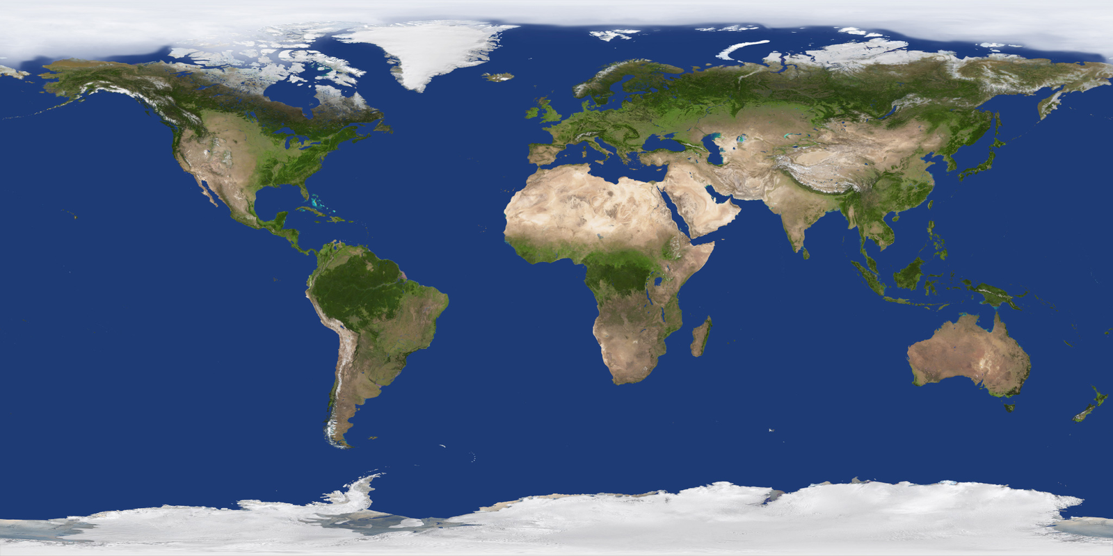
UV mapping consists of “unfolding” the 3D surface onto a 2D plane. This unfolding necessarily introduces deformations in length and in angle for any surface whose Gaussian curvature is nonzero.
In particular, it is impossible to map a planar image onto a sphere without distortion. This is a fundamental result of differential geometry: Gaussian curvature is an intrinsic invariant of the surface (Gauss’s theorema egregium). A sphere has constant positive Gaussian curvature (\(K = 1/R^2\)), while a plane has zero curvature (\(K = 0\)). No distortion without stretching can transform one into the other.
Only the developable surfaces (Gaussian curvature zero, such as cylinders and cones) can be unfolded without distortion. In practice, one seeks to minimize deformations during UV unfolding, accepting a trade-off between the distortion of angles (conformal) and the distortion of areas (authalic). The following figure shows a typical case of deformation on a sphere.
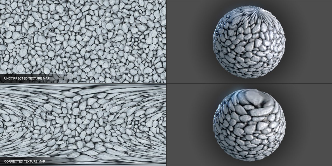
Déformation lors du placage d'une texture sur une sphère : étirement aux pôles.
Beyond color (diffuse map), textures are used to store many types of information about the surface:
Texture coordinates are stored as a vertex attribute, in the same way as positions and normals:
std::vector<vec2> uv = { uv_0, uv_1, uv_2, ... };On the C++/OpenGL side, the texture is loaded and sent to the GPU:
// Chargement de l'image
int width, height, channels;
unsigned char* data = stbi_load("texture.png", &width, &height, &channels, 4);

// Création de la texture OpenGL
GLuint texture_id;
glGenTextures(1, &texture_id);
glBindTexture(GL_TEXTURE_2D, texture_id);
glTexImage2D(GL_TEXTURE_2D, 0, GL_RGBA, width, height, 0,
             GL_RGBA, GL_UNSIGNED_BYTE, data);

// Activation dans le fragment shader (unité de texture 0)
glActiveTexture(GL_TEXTURE0);
glBindTexture(GL_TEXTURE_2D, texture_id);
glUniform1i(glGetUniformLocation(shader, "texture_image"), 0);During rendering, the fragment shader receives the texture
coordinates \((u, v)\) that are
barycentrically interpolated between the three vertices of the current
triangle. It then reads the color from the texture image at that
position using the texture() function:
uniform sampler2D texture_image;  // la texture, envoyée depuis le CPU

in vec2 fragment_uv;              // coordonnées interpolées
out vec4 FragColor;

void main() {
    vec4 color = texture(texture_image, fragment_uv);
    FragColor = color;
}
The variable sampler2D represents a reference to a
texture stored in VRAM. The function texture(sampler, uv)
performs the sampling: it converts the normalized
coordinates \((u, v) \in [0, 1]^2\) to
pixel coordinates in the image, and then returns the corresponding
color.
The interpolated coordinates \((u, v)\) rarely land exactly at the center of a texture pixel (called a texel). The GPU must therefore interpolate between neighboring texels. This process is called texture filtering. It occurs in two cases:
The most common filtering modes are :
GL_NEAREST) : selects the
nearest texel. Pixelated rendering but fast. Useful for a pixel-art
style.GL_LINEAR) : bilinearly
interpolates between the 4 closest texels. Smooth rendering, standard
for magnification.GL_LINEAR_MIPMAP_LINEAR)
: bilinear interpolation + interpolation between two mipmap levels (see
below). Standard for minification.OpenGL configuration:
glTexParameteri(GL_TEXTURE_2D, GL_TEXTURE_MAG_FILTER, GL_LINEAR);
glTexParameteri(GL_TEXTURE_2D, GL_TEXTURE_MIN_FILTER, GL_LINEAR_MIPMAP_LINEAR);
Mipmaps are precomputed versions of the texture at decreasing resolutions (each level halves the resolution). During minification, the GPU selects the mipmap level whose resolution is most suitable for the size of the triangle on screen, and interpolates if necessary.
For a texture of \(1024 \times 1024\), the mipmap chain contains the levels: \(1024^2\), \(512^2\), \(256^2\), …, \(2^2\), \(1^2\) (i.e., 11 levels). The total memory footprint is only \(\frac{4}{3}\) of the original texture.
Mipmaps reduce the aliasing (flickering of textures viewed from afar) and improve performance (the distant textures are read at lower-resolution levels, better utilized by the GPU’s memory cache).
Automatic generation in OpenGL :
glGenerateMipmap(GL_TEXTURE_2D);When texture coordinates exit the interval \([0, 1]\), the behavior depends on the wrapping mode:
GL_REPEAT) : the texture
repeats indefinitely. The coordinate \(u =
2.3\) is interpreted as \(u =
0.3\). Useful for tiling textures (bricks, grass, etc.).GL_MIRRORED_REPEAT) :
the texture repeats while alternating its orientation, avoiding visible
seams at the edges.GL_CLAMP_TO_EDGE) :
coordinates outside \([0, 1]\) are
clamped to the edge of the texture. Out-of-range pixels take the color
of the closest edge.OpenGL configuration:
glTexParameteri(GL_TEXTURE_2D, GL_TEXTURE_WRAP_S, GL_REPEAT);
glTexParameteri(GL_TEXTURE_2D, GL_TEXTURE_WRAP_T, GL_REPEAT);All textures (color, normals, specular, etc.) share the same UV
coordinates and use the same sampling mechanism. They are simply read
from different sampler2Ds in the fragment shader:
uniform sampler2D diffuse_map;
uniform sampler2D normal_map;
uniform sampler2D specular_map;

void main() {
    vec3 color    = texture(diffuse_map,  fragment.uv).rgb;
    vec3 normal   = texture(normal_map,   fragment.uv).rgb * 2.0 - 1.0;
    float spec    = texture(specular_map, fragment.uv).r;
    // ...
}A skybox is a textured box representing the distant environment (sky, landscape). It is always centered on the camera’s position, which gives the impression of an infinite landscape, as shown below.
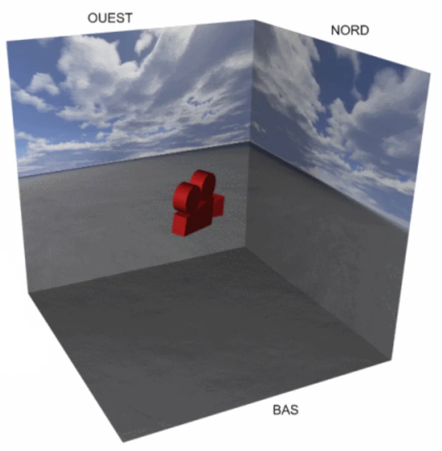
The implementation principle is as follows:
void display() {
    glDepthMask(GL_FALSE);   // désactiver l'écriture dans le depth buffer
    draw(skybox, environment);

    glDepthMask(GL_TRUE);    // réactiver l'écriture
    // dessiner les autres objets ...
}The environment mapping simulates the reflection of the environment (skybox) on a shiny surface. This gives the impression that the object reflects the world around it.
The principle, illustrated below, is to compute, for each fragment, the reflection direction of the view vector with respect to the normal, and then read the corresponding color from the skybox texture.

vec3 V = normalize(camera_position - fragment.position);
vec3 R_skybox = reflect(-V, N);
vec4 color_env = texture(image_skybox, R_skybox);The normal mapping consists of modifying the surface normals using an image (the normal map) to simulate geometric details finer than the triangles of the mesh. The real geometry of the triangle does not change: only the normal used in the illumination calculation is modified, which yields the illusion of relief visible in the following comparison.

The normals of a normal map are not stored in world coordinates (which would depend on the object’s orientation), but in a frame local to the triangle called the tangent space \((T, B, N)\) :
This frame is defined by the texture coordinates \((u, v)\) and the positions of the triangle’s vertices:
\[ \begin{cases} p_0 - p_1 = (u_0 - u_1) \, T + (v_0 - v_1) \, B \\ p_2 - p_1 = (u_2 - u_1) \, T + (v_2 - v_1) \, B \\ N = T \times B \end{cases} \] This system of two vector equations (i.e., 6 scalar equations) allows solving \(T\) and \(B\) (6 unknowns). In matrix notation, for the x components, for example:
\[ \begin{pmatrix} T_x \\ B_x \end{pmatrix} = \frac{1}{(u_0 - u_1)(v_2 - v_1) - (u_2 - u_1)(v_0 - v_1)} \begin{pmatrix} v_2 - v_1 & -(v_0 - v_1) \\ -(u_2 - u_1) & u_0 - u_1 \end{pmatrix} \begin{pmatrix} (p_0 - p_1)_x \\ (p_2 - p_1)_x \end{pmatrix} \] And likewise for the components \(y\) and \(z\). The vectors \(T\) and \(B\) are then normalized.
Each pixel of the normal map stores a perturbed normal with components \((r, g, b) \in [0, 1]^3\), encoding the components in tangent space to [-1, 1]:
\[ n_{\text{tangent}} = 2 \begin{pmatrix} r \\ g \\ b \end{pmatrix} - \begin{pmatrix} 1 \\ 1 \\ 1 \end{pmatrix} \] The blue component \(b\) corresponds to the direction of the geometric normal \(N\). That’s why normal maps appear bluish: most normals are close to \((0, 0, 1)\) in tangent space, which yields \((0.5, 0.5, 1.0)\) in RGB. This encoding can be observed in the images below.
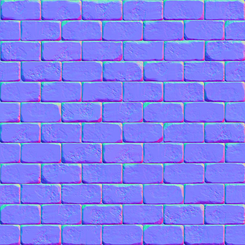
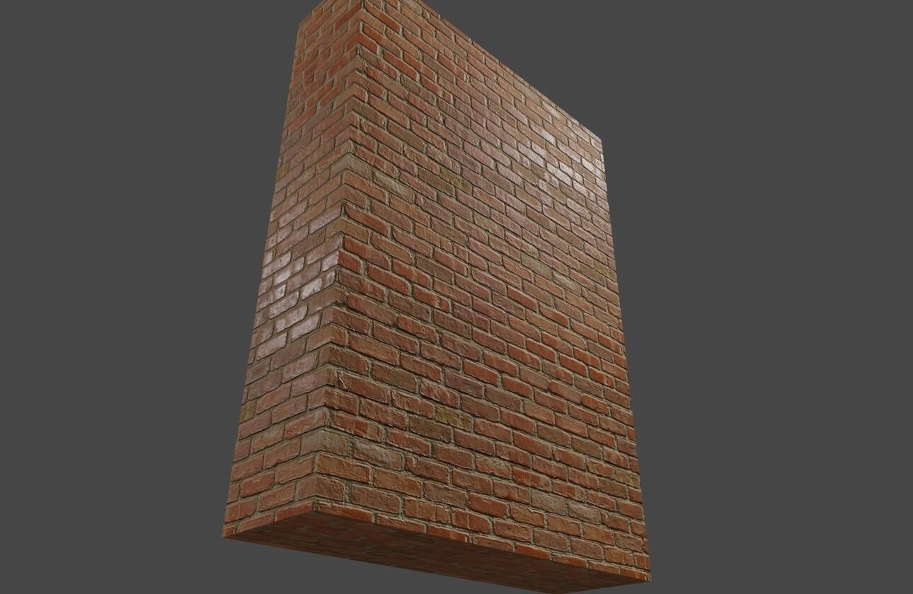
Normal map : les normales sont encodées en couleur dans l'espace tangent (gauche). Application sur un mur en briques (droite).
The final normal vector in world coordinates is obtained by a change of basis:
\[ n_{\text{world}} = \text{TBN} \times n_{\text{tangent}} = T \cdot n_x + B \cdot n_y + N \cdot n_z \] where \(\text{TBN} = (T \mid B \mid N)\) is the 3×3 matrix whose columns are the vectors of the tangent frame.
Vertex shader: calculation of the tangent frame and passing to the fragment shader.
layout(location = 0) in vec3 vertex_position;
layout(location = 1) in vec3 vertex_normal;
layout(location = 2) in vec2 vertex_uv;
layout(location = 3) in vec3 vertex_tangent;

out struct fragment_data {
    vec3 position;
    vec2 uv;
    mat3 TBN;
} fragment;

uniform mat4 model;
uniform mat4 view;
uniform mat4 projection;

void main() {
    vec4 pos_world = model * vec4(vertex_position, 1.0);
    mat3 normalMatrix = mat3(transpose(inverse(model)));

    vec3 T = normalize(normalMatrix * vertex_tangent);
    vec3 N = normalize(normalMatrix * vertex_normal);
    vec3 B = cross(N, T);

    fragment.position = pos_world.xyz;
    fragment.uv = vertex_uv;
    fragment.TBN = mat3(T, B, N);

    gl_Position = projection * view * pos_world;
}
Fragment shader : sampling the normal map and illumination calculation.
in struct fragment_data {
    vec3 position;
    vec2 uv;
    mat3 TBN;
} fragment;

uniform sampler2D normal_map;
uniform vec3 light_position;

out vec4 FragColor;

void main() {
    // Lire la normale dans la normal map et la convertir de [0,1] à [-1,1]
    vec3 n_tangent = texture(normal_map, fragment.uv).rgb * 2.0 - 1.0;

    // Transformer vers l'espace monde
    vec3 N = normalize(fragment.TBN * n_tangent);

    // Illumination avec la normale perturbée
    vec3 L = normalize(light_position - fragment.position);
    float diffuse = max(dot(N, L), 0.0);

    // ...
}
The advantage of the tangent space is that the same normal map can be reused on different objects or different parts of the same object, regardless of their orientation in the world.
Parallax mapping goes beyond texture coordinates themselves according to a height map (height map). While normal mapping only modifies the illumination (the silhouette remains flat), parallax mapping creates an impression of geometric displacement: the high areas appear to come forward and the low areas recede, especially when viewing the surface at a grazing angle.
Consider a fragment on a flat surface. Without parallax mapping, we would sample the texture at the coordinates \((u, v)\) for this fragment. But if the surface actually had relief, the viewing ray would have intersected the surface at a different point, horizontally offset. Parallax mapping approximates this offset, as shown in the diagram below.

Let \(V\) be the view vector expressed in tangent space and \(h\) the height read from the height map at the current point. The texture coordinate offset is:
\[ (u', v') = (u, v) + h \cdot \frac{(V_x, V_y)}{V_z} \] The division by \(V_z\) amplifies the offset at grazing angles (when \(V_z\) is small), which corresponds to the expected physical behavior: parallax is more noticeable at oblique angles.
Fragment shader with parallax mapping :
in struct fragment_data {
    vec3 position;
    vec2 uv;
    mat3 TBN;
} fragment;

uniform sampler2D diffuse_map;
uniform sampler2D height_map;
uniform sampler2D normal_map;
uniform vec3 camera_position;
uniform float height_scale;  // contrôle l'amplitude du relief (~0.05-0.1)

out vec4 FragColor;

void main() {
    // Vecteur de vue dans l'espace tangent
    vec3 V_world = normalize(camera_position - fragment.position);
    vec3 V_tangent = normalize(transpose(fragment.TBN) * V_world);

    // Lire la hauteur et calculer le décalage
    float h = texture(height_map, fragment.uv).r;
    vec2 uv_offset = h * height_scale * V_tangent.xy / V_tangent.z;
    vec2 uv_parallax = fragment.uv + uv_offset;

    // Utiliser les coordonnées décalées pour la texture et la normal map
    vec3 color = texture(diffuse_map, uv_parallax).rgb;
    vec3 n_tangent = texture(normal_map, uv_parallax).rgb * 2.0 - 1.0;
    vec3 N = normalize(fragment.TBN * n_tangent);

    // Illumination avec la normale et la couleur décalées
    // ...
}Simple parallax mapping is a first-order approximation that works well for low-relief surfaces. For more pronounced reliefs, it produces artifacts (slippages, distortions). The Steep Parallax Mapping (or Parallax Occlusion Mapping) improves quality by stepping through the view ray step-by-step across the height map:
vec2 steep_parallax(vec2 uv, vec3 V_tangent, float height_scale) {
    const int num_steps = 32;
    float step_size = 1.0 / float(num_steps);
    float current_depth = 0.0;
    vec2 delta_uv = V_tangent.xy / V_tangent.z * height_scale / float(num_steps);

    vec2 current_uv = uv;
    float current_height = texture(height_map, current_uv).r;

    for(int i = 0; i < num_steps; i++) {
        if(current_depth >= current_height) break;
        current_uv += delta_uv;
        current_height = texture(height_map, current_uv).r;
        current_depth += step_size;
    }

    return current_uv;
}
This method is more expensive (one texture fetch per step), but yields visually convincing results even for substantial reliefs, with proper handling of the self-occlusion of relief details.
Many visual phenomena — smoke, fire, water spurting, explosions, sparks, snow — do not have a sharp and well-defined surface. Unlike a solid object (a character, a building), these effects are diffuse: they are composed of a large number of tiny elements that evolve in a partially random manner. Attempting to model them with a classical mesh would be both costly and ill-suited, as their shape constantly changes and does not correspond to a stable geometric surface.
A particle system meets this need. The concept, introduced by William Reeves in 1983 for the effects of the film Star Trek II, rests on a simple idea: model these phenomena as a set of independent elements (the particles), each following a simple behavior rule. It is the collective behavior of thousands of particles that produces the desired visual effect.
Each particle is characterized by:
The particle lifecycle follows four phases. The emission: the particle is created at an initial position with an initial velocity and attributes (possibly random). The simulation: at each time step, its position is updated according to a motion equation, and its attributes may evolve (for example, transparency gradually increases to simulate the dissipation of smoke). The death: when the life duration is elapsed, the particle is deactivated. The recycling: in practice, we pre-allocate an array of particles of fixed size. When a particle dies, its slot is reused for a new particle, avoiding costly dynamic allocations.
The geometric representation simplest is the sphere: each particle is drawn as a small sphere in the 3D scene. This approach is intuitive but expensive in geometry for a large number of particles. For more detailed and more performant effects, one uses billboards (see next section).
The most common case is free fall under the effect of gravity. In physics, Newton’s second law gives the acceleration \(a = g\) (constant), which, by double integration, provides the equation of motion :
\[ p(t) = \frac{1}{2} \, g \, t^2 + v_0 \, t + p_0 \] with :
This equation describes a parabola: the particle rises (if \(v_0\) has a positive vertical component), slows under the effect of gravity, then falls. It is exactly the trajectory of a projectile.
To create a fountain or jet effect, we introduce randomization in the initial conditions. It is this variability among particles that gives a natural look to the ensemble: if all particles had exactly the same parameters, they would all follow the same trajectory and the effect would be visually poor.
// Exemple : émission d'une particule
vec3 p0 = emitter_position + rand_vec3(-0.1f, 0.1f);
vec3 v0 = vec3(0, 5, 0) + rand_vec3(-1.0f, 1.0f);
float lifetime = rand(1.0f, 3.0f);
Velocity is obtained by differentiation:
\[ v(t) = g \, t + v_0 \] At each time step, particles whose lifetime has expired are removed, and new particles are emitted. In practice, the emitter produces a constant flux (for example, 100 particles per second), which maintains a stable number of active particles in the scene.
When a particle encounters an obstacle (for example the ground at \(y = 0\)), it is possible to simulate a bounce. The idea is to detect the exact instant of collision, then restart the simulation with a modified velocity. The principle is as follows :
\[ p_y(t_i) = \frac{1}{2} g_y \, t_i^2 + v_{0,y} \, t_i + p_{0,y} = 0 \] 2. Calculation of impact velocity :
\[ v(t_i) = g \, t_i + v_0 \] 3. Inversion of the normal component : after the bounce, the component of velocity perpendicular to the surface is inverted and attenuated by a coefficient of restitution \(\epsilon \in [0, 1]\) :
\[ v_y^{\text{après}} = -\epsilon \, v_y(t_i) \] The coefficient \(\epsilon\) controls the rebound behavior: \(\epsilon = 1\) corresponds to a perfectly elastic rebound (the particle leaves with the same energy), while \(\epsilon = 0\) means that the particle is totally absorbed by the surface (it stops). In practice, intermediate values (\(\epsilon \approx 0.6\text{-}0.8\)) are used to achieve a realistic effect.
The particle then leaves with this new velocity as the initial condition, producing a piecewise trajectory. By repeating this process, one obtains a sequence of rebounds with decreasing amplitude until the particle comes to rest or its lifetime expires.
This principle generalizes to arbitrary obstacles: for an oblique plane defined by its normal \(\hat{n}\), the reflected component is the projection of the velocity onto this normal: \(v^{\text{after}} = v(t_i) - (1 + \epsilon)(v(t_i) \cdot \hat{n})\,\hat{n}\).
Trajectories are not necessarily constrained by physics. In computer graphics, the objective is often to produce a convincing visual effect rather than a faithful simulation. We can thus define arbitrary procedural movements, guided by aesthetics rather than Newton’s laws.
Some classic examples:
The difference with physical simulation is the artistic freedom: the designer can adjust the movement parameters to obtain exactly the desired effect, without being constrained by realism. A particle vortex in a video game does not need to obey the Navier-Stokes equations to be visually convincing.
Rendering each particle as a 3D sphere is expensive: a smooth sphere requires hundreds of triangles, and a system of 10 000 particles would then represent millions of triangles. Rather than drawing 3D geometry, we use billboards (or impostors): textured quadrilaterals that always face the camera.
The idea is to fool the eye: since a quadrangle oriented toward the camera always appears face-on (without perspective revealing itself), it is enough to apply a realistic texture to give the illusion of a more complex object. The principle rests on three elements:
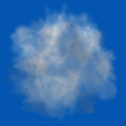
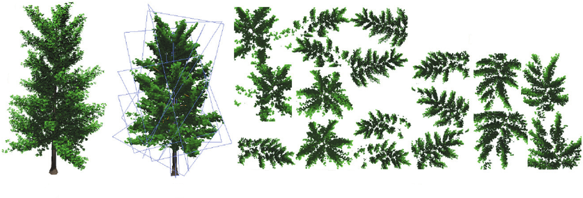
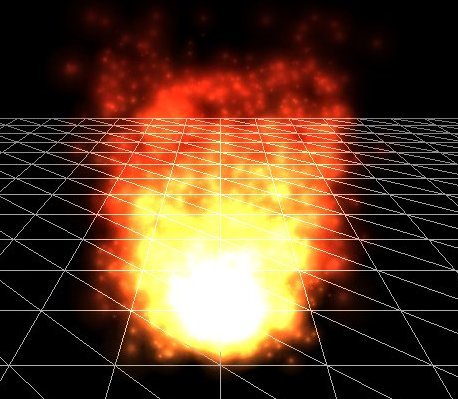
Billboards : texture de fumée avec canal alpha (gauche), arbre composé de quadrangles texturés avec ses textures de feuillage (centre), effet de feu obtenu par accumulation de billboards (droite).
Two types of billboards are distinguished according to their axis of freedom:
Several extensions of the concept exist :
The main advantage is the cost/quality ratio: a billboard requires only 4 vertices (2 triangles) per particle, versus hundreds for a full 3D geometry. For a system of 10,000 particles, that represents 20,000 triangles instead of several millions.
The rendering of billboards relies on transparency, which is a fundamentally difficult problem in rasterization. In ray tracing, transparency is natural: a ray that traverses a semi-transparent object continues its path and accumulates the colors of the encountered objects. In rasterization, however, each triangle is drawn independently into the framebuffer, without knowledge of the triangles that will be drawn subsequently. Thus, the management of transparency requires explicit mechanisms. There is no perfect solution, but several complementary approaches.
Transparency in OpenGL works by color blending (blending): the color of the current fragment is combined with the color already present in the framebuffer, using the alpha channel (\(\alpha\)) as a weighting factor.
The activation is performed explicitly:
glEnable(GL_BLEND);
glBlendFunc(GL_SRC_ALPHA, GL_ONE_MINUS_SRC_ALPHA);
// ... appels de dessin des objets transparents ...
glDisable(GL_BLEND);
The resulting blending formula is:
\[ C_{\text{new}} = \alpha \cdot C_{\text{current}} + (1 - \alpha) \cdot C_{\text{previous}} \] with:
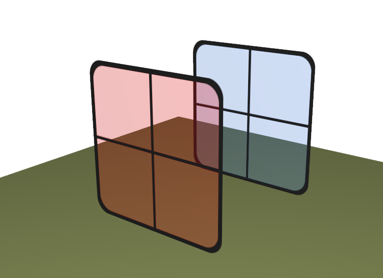
Point important: the drawing order matters. The color \(C_{\text{previous}}\) depends on what has been drawn before the current fragment. If two transparent objects overlap, the result depends on the order in which they were rendered. This is a major difference from opaque objects, for which the depth buffer guarantees a correct result regardless of the drawing order.
There exist other blending modes, defined by different combinations
of glBlendFunc. For example, the additive blending
(GL_SRC_ALPHA, GL_ONE) adds colors without attenuating the
destination: \(C_{\text{new}} = \alpha \cdot
C_{\text{current}} + C_{\text{previous}}\). This mode is
particularly suited for luminous effects (fire, sparks, lasers), because
colors accumulate and produce regions of high brightness.
To obtain correct rendering of transparent objects, one must respect a fundamental constraint: transparent objects must be drawn from farthest to nearest (back-to-front). Indeed, the blending formula blends the color of the current fragment with what is already in the framebuffer. For the result to be physically coherent (a semi-transparent red object in front of a blue object), the blue object (the farthest) must already be in the framebuffer when drawing the red object (the nearest).
The standard approach follows these steps :
Draw all opaque objects normally (with the depth buffer enabled for reading and writing). This step fills the depth buffer, which will prevent transparent objects from appearing in front of the opaque objects that occlude them.
Enable blending and disable writing to the depth buffer (but not reading) :
glEnable(GL_BLEND);
glBlendFunc(GL_SRC_ALPHA, GL_ONE_MINUS_SRC_ALPHA);
glDepthMask(false); // désactiver l'écriture dans le depth buffer// Calcul de la profondeur pour le tri
vec4 p_proj = projection * modelview * vec4(position, 1.0);
float z_depth = p_proj.z / p_proj.w;Draw the transparent objects in sorted order (from farthest to nearest).
Restore the state :
glDisable(GL_BLEND);
glDepthMask(true);
The complete code of the algorithm:
// 1. Objets opaques
draw_opaque_objects();

// 2-3. Objets transparents
glEnable(GL_BLEND);
glBlendFunc(GL_SRC_ALPHA, GL_ONE_MINUS_SRC_ALPHA);
glDepthMask(false);

sort_by_depth(transparent_objects, camera_position);  // du plus loin au plus proche

for(auto& obj : transparent_objects) {
    draw(obj);
}

glDisable(GL_BLEND);
glDepthMask(true);
Disabling writing to the depth buffer is essential: a transparent object should not occlude the objects located behind it. By contrast, the reading of the depth buffer remains active, which prevents transparent objects from being drawn in front of the opaque objects that occlude them.
Two common mistakes in transparent rendering:
Error 1: depth buffer writing without sorting. If writing to the depth buffer remains enabled and the objects are not sorted, a nearby transparent object can write to the depth buffer and prevent rendering of objects behind it. The depth buffer “blocks” the farther fragments, even if the foreground object is semi-transparent and should allow what lies behind to be seen. The result is pronounced visual artifacts: pieces of objects disappear incoherently, with “holes” in the scene that depend on the order in which triangles are submitted to the GPU.
Error 2: no sorting, depth buffer writing disabled. Without sorting but with depth buffer writing disabled, transparent objects are blended in an arbitrary order. For objects whose colors are close and whose shapes are diffuse (smoke, clouds, fog), the blending order has little visual impact and the result is approximately acceptable. This approach is sometimes used in practice to avoid the cost of sorting — which can be significant for thousands of particles — when visual quality does not need to be perfect. However, for transparent objects with vivid and high-contrast colors (stained glass, crystals), the lack of sorting produces visible artifacts.
For billboards whose texture is either entirely opaque, or entirely transparent (no semi-transparency), there exists a simpler approach: the discard in the fragment shader.
The keyword discard stops the execution of the fragment
shader: nothing is written to the framebuffer nor to the depth buffer
for this fragment. It suffices to test the alpha value of the
texture:
uniform sampler2D image_texture;
in vec2 uv;
out vec4 FragColor;

void main() {
    vec4 color = texture(image_texture, uv);
    float alpha_limit = 0.6;

    if(color.a < alpha_limit) {
        discard;  // fragment entièrement transparent : on l'ignore
    }

    FragColor = color;
}
Advantages :
Disadvantages :
alpha_limit threshold creates a
sharp boundary).A particle system can contain thousands, or even hundreds of
thousands of elements sharing the same geometry (for example a
quadrilateral for a billboard) but with different parameters (position,
color, size). The naive approach consists of calling
glDrawElements for each particle:
for(int k = 0; k < N; ++k) {
    update_uniforms(k);   // position, couleur, taille...
    draw(shape);          // glDrawElements(...)
}
This loop is very inefficient. To understand why,
one must consider the CPU/GPU architecture: each call to
glDrawElements does not simply trigger rendering. It causes
a synchronization between the CPU and the GPU: the
OpenGL driver must validate the current state (active shader, uniforms,
textures, buffers), prepare the command, and send it to the GPU. This
per-call overhead is roughly constant, regardless of the geometry size.
The graph below, taken from NVIDIA’s documentation, illustrates the
relative cost of the different state changes: even the least expensive
operations (updating uniforms) are limited to about 10 million per
second.
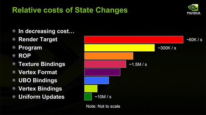
For 15,000 particles composed of 50 triangles each, this represents 15,000 draw calls and 750,000 vertices, but it is the number of calls (and not the number of vertices) that constitutes the CPU bottleneck.
Instancing resolves this problem by replacing the \(N\) draw calls with a single call that asks the GPU to draw \(N\) copies of the same geometry:
drawInstanced(shape, N); // glDrawElementsInstanced(..., N)Instancing rests on two elements:
CPU side: replacement of glDrawElements
by glDrawElementsInstanced:
// Au lieu de :
// glDrawElements(GL_TRIANGLES, count, GL_UNSIGNED_INT, 0);

// On utilise :
glDrawElementsInstanced(GL_TRIANGLES, count, GL_UNSIGNED_INT, 0, N);
where \(N\) is the number of instances (particles) to be drawn.
Shader side: the built-in variable
gl_InstanceID allows differentiating each instance. It
contains the index of the current instance (from 0 to \(N-1\)) and enables reading the parameters
specific to each particle:
// Vertex shader
uniform vec3 positions[MAX_PARTICLES];  // ou via un SSBO / texture
uniform vec3 colors[MAX_PARTICLES];

void main() {
    vec3 offset = positions[gl_InstanceID];
    vec3 color  = colors[gl_InstanceID];

    gl_Position = projection * view * vec4(vertex_position + offset, 1.0);
    // ...
}
Performance gains are substantial. For example:
The gain is significant because instancing eliminates the CPU bottleneck: instead of 15 000 round trips CPU→GPU, one suffices, and the GPU — whose architecture is designed for massively parallel processing — can process the millions of resulting vertices without difficulty.
Instancing is the standard technique for any rendering requiring a large number of copies of the same geometry: particles, vegetation (grass, trees), crowds, asteroids, etc. For even more advanced cases (variable number of instances, complex parameters), one can replace uniform arrays with Shader Storage Buffer Objects (SSBOs) or data textures, which are not limited in size like uniform arrays.
In computer graphics, the creation of natural shapes (terrains, clouds, stone textures, wood textures, water textures) poses a challenge: these shapes are too complex and irregular to be manually modeled, but they are not purely random either — they possess a recognizable structure. A mass of white noise (independent random values at each pixel) bears no resemblance to anything natural; a texture painted by hand is costly to produce and limited in resolution.
Procedural noise addresses this need: a mathematical function that generates a pseudo-random pattern on demand, with controlled properties:
The most common procedural noises are illustrated below.
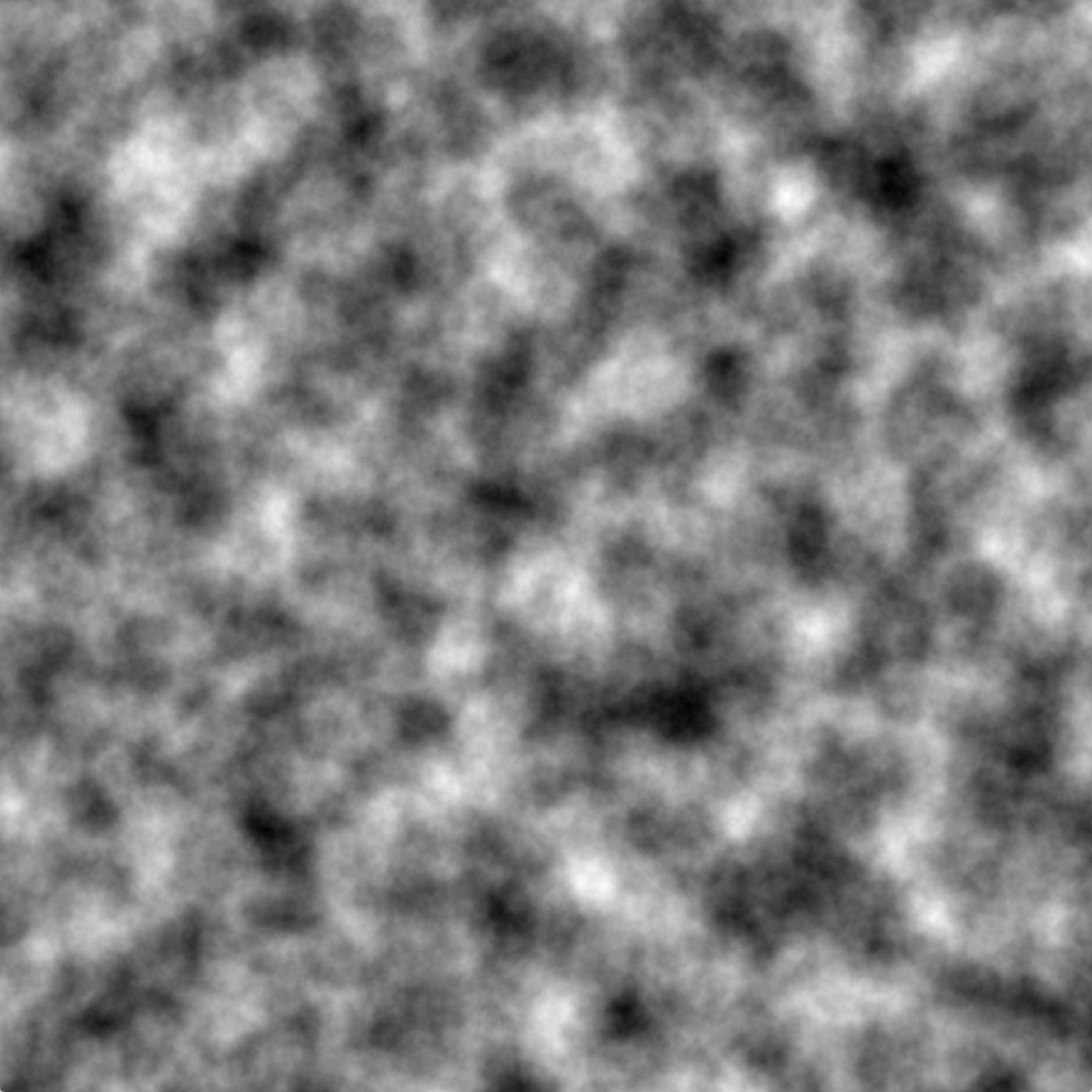
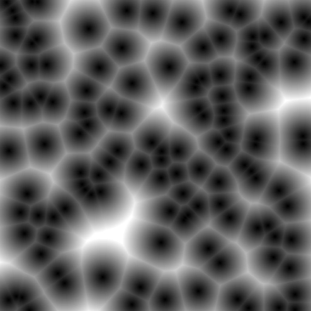

Exemples de bruits procéduraux : Perlin (gauche), Worley (centre), Flow (droite).
Procedural noises are used for the generation of terrains, textures, animations, and more generally for any complex form requiring a natural appearance without explicit data storage.
The construction of 1D procedural noise rests on two ingredients:
float hash(float n) {
    return fract(sin(n) * 1e4);
}
This function exploits the fact that \(\sin(n) \times 10^4\) yields values whose
decimals vary in an apparently chaotic way from one integer to the next,
and fract extracts the fractional part to obtain a result
in \([0, 1]\).
The algorithm to evaluate \(f(x)\) is:

The resulting function is:
This principle generalizes directly to 2D and 3D. In 2D, we use a grid of integers \((i, j)\) with a hash value \(h(i, j)\) at each node, and we bilinearly interpolate within each cell. In 3D, the interpolation is trilinear. The computational cost increases with dimension (4 hash evaluations in 2D, 8 in 3D), but remains reasonable for real-time computation.
A continuous noise with a fixed frequency produces a pattern too regular to simulate natural shapes. Nature presents details at all scales: a mountain viewed from afar has a jagged silhouette; as you approach, one discovers ridges, then rocks, then pebbles, then grains of sand. Each level of zoom reveals new details. Similarly, a coastline is carved at the kilometer, meter and centimeter scale. A cloud has swirls at all sizes.
The concept of fractal formalizes this idea: a shape is fractal if it exhibits a self-similarity, that is, its structure repeats (approximately) at different scales. Classic examples are the Koch snowflake (whose perimeter increases at each iteration but whose area remains bounded), the Sierpinski triangle, or natural shapes such as the Romanesco broccoli whose spirals repeat at several levels of scale.

The interest of fractals in computer graphics is that a simple rule applied recursively can produce forms of great visual complexity, reminiscent of natural structures. However, classical mathematical fractals (Mandelbrot, Sierpinski) are difficult to control for artistic use. In practice, one uses instead the sum of noises at different frequencies, as in Perlin noise.
The Perlin noise (Ken Perlin, An Image Synthesizer, SIGGRAPH 1985) is the first procedural noise algorithm and remains the most widely used in computer graphics. This contribution earned him a Technical Academy Award in 1997. Its central idea is to reproduce the fractal principle of nature by summing pseudo-random functions with increasing frequencies and decreasing amplitudes:
\[ P(x) = \sum_{k=0}^{N} \alpha^k \, f(\omega^k \, x) \] with:
The figure below shows the decomposition into octaves: the first octave gives the overall shape, the following ones add increasingly finer details.
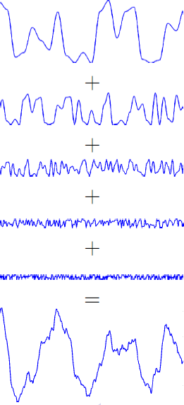
In 2D, the formula becomes:
\[ P(u, v) = \sum_{k=0}^{N} \alpha^k \, f(2^k \, u, \, 2^k \, v) \] The images below illustrate the progressive accumulation of octaves in 2D.
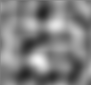

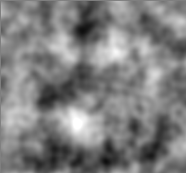
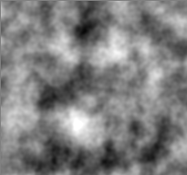

Accumulation des octaves du bruit de Perlin en 2D : de 1 octave (gauche) à 5 octaves (droite).
The typical parameters are \(N \approx 5\text{-}9\), \(\alpha \approx 0.3\text{-}0.6\) and \(\omega = 2\). Adjusting these parameters allows control over the appearance of the noise: more detail with larger \(N\), more pronounced details with \(\alpha\) close to 1.
Perlin noise is used to generate virtually all complex forms in computer graphics. Its simplicity and versatility explain its success: by modifying the parameters or by combining the noise with other mathematical operations, one obtains a wide variety of effects.
Procedural terrain: the most direct application is to use the noise as a height map (height map). We define a flat surface \((x, y)\) and we vertically displace each point according to the value of the noise:
\[ z(x, y) = P(x, y) \] The height of each point on the terrain is directly determined by the value of the noise. The low frequencies (first octaves) define the large-scale structures (valleys, mountains), while the high frequencies add the details (rocks, asperities). The result resembles a natural mountainous landscape, as real terrains are also formed by multi-scale processes (tectonics, erosion, freezing).
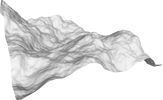
Ridge texture (ridge) : by taking the absolute value of the base noise :
\[ \text{ridge}(x) = \sum_k \alpha^k \, |f(\omega^k \, x)| \] The absolute value creates folds (cusps) at the points where the noise crosses zero: instead of a smooth positive-to-negative transition, one gets a sharp V. These folds form sharp edges that resemble mountain crests, the veins of a leaf, or the grain of wood.
Marble texture: by using the noise as a perturbation of a sinusoidal function:
\[ \text{marble}(x) = \sin\!\Big(x + \sum_k \alpha^k \, |f(\omega^k \, x)|\Big) \] The idea is that the sine wave naturally produces regular bands (like the layers in stone), and the noise irregularly distorts these bands. The undulations of the sine wave, perturbed by the noise, produce a veined pattern similar to marble. By adjusting the amplitude of the perturbation, one controls the irregularity of the veins.
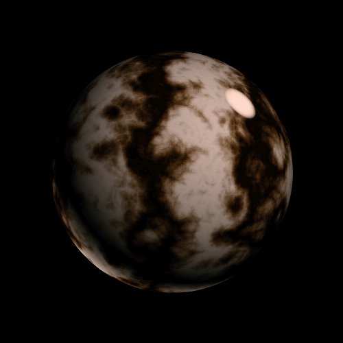
Animated textures: noise can be extended into time to create animations:
These techniques are omnipresent in video games and films: the surface of water, the movement of clouds, the deformation of lava, the effects of thermal distortion are generally based on animated Perlin noise variants.
The original Perlin algorithm has certain limitations that have motivated successive improvements.
In the original algorithm (called value noise), each grid node stores a pseudo-random scalar value \(h(i, j) \in [0, 1]\), and we interpolate these values. The problem is that if two neighboring nodes have values close to each other (for example \(h = 0.7\) and \(h = 0.72\)), the noise varies very little in this region, producing a lower local frequency than expected. The frequency of the noise is therefore irregular from one cell to the next.
The gradient noise (Ken Perlin, 2002) corrects this problem by associating to each node \((i, j)\) a gradient vector pseudo-random \(g_{i,j}\) (a unit vector in a random direction) rather than a scalar. The algorithm to evaluate the noise at a point \(p = (x, y)\) is :
The key property is that the dot product \(g_{i,j} \cdot d\) is zero at the node itself (because \(d = 0\) at the node). The noise therefore passes through zero at every grid node, which guarantees exactly one oscillation per unit in each direction. The frequency is thus perfectly controlled and homogeneous over the entire domain, which yields a visually more regular result than the value noise.
In pseudocode :
float gradient_noise(float x, float y) {
    int i = floor(x), j = floor(y);
    float u = x - i, v = y - j;  // coordonnées locales dans [0,1]²

    // Gradients aux 4 coins
    vec2 g00 = gradient(i,   j  );
    vec2 g10 = gradient(i+1, j  );
    vec2 g01 = gradient(i,   j+1);
    vec2 g11 = gradient(i+1, j+1);

    // Produits scalaires (contribution de chaque coin)
    float d00 = dot(g00, vec2(u,   v  ));
    float d10 = dot(g10, vec2(u-1, v  ));
    float d01 = dot(g01, vec2(u,   v-1));
    float d11 = dot(g11, vec2(u-1, v-1));

    // Interpolation smoothstep
    float sx = smoothstep(u), sy = smoothstep(v);
    return mix(mix(d00, d10, sx), mix(d01, d11, sx), sy);
}The Simplex Noise (Ken Perlin, 2001) replaces the Cartesian grid with a tiling of simplices. A simplex is the simplest polytope in dimension \(d\): a line segment in 1D, a triangle in 2D, a tetrahedron in 3D. In 2D, space is thus tiled by equilateral triangles instead of squares.
The algorithm comprises three main steps:
1. Localization of the simplex (skewing). To determine in which triangle a point \((x, y)\) lies, one applies a deformation transformation (skew) that transforms the grid of triangles into a square grid, facilitating localization:
\[ (x', y') = \Big(x + \frac{\sqrt{3} - 1}{2}(x + y), \;\; y + \frac{\sqrt{3} - 1}{2}(x + y)\Big) \] In the distorted space, we identify the square \((\lfloor x' \rfloor, \lfloor y' \rfloor)\), then determine in which triangle of the square we are (upper or lower diagonal) by testing whether \(x' - \lfloor x' \rfloor > y' - \lfloor y' \rfloor\).
2. Calculation of contributions. Each simplex has \(d + 1\) vertices (3 in 2D). For each vertex, we compute a local contribution using a radial attenuation function instead of interpolation:
\[ \text{contribution}_k = \max(0, \; r^2 - \|d_k\|^2)^4 \cdot (g_k \cdot d_k) \] where \(d_k\) is the displacement vector from vertex \(k\) to the evaluated point, \(g_k\) is the pseudo-random gradient at the vertex, and \(r\) is an influence radius (typically \(r^2 = 0.5\) in 2D). The fourth power ensures a fast and smooth decay, with \(C^2\) continuity.
3. Summation. The final noise is the sum of the contributions from the \(d + 1\) vertices:
\[ \text{simplex}(p) = \sum_{k=0}^{d} \text{contribution}_k \] The advantages over grid-based noise are as follows:
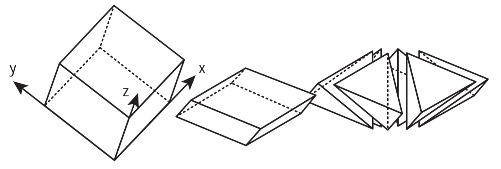
For further reading: A. Lagae et al., A Survey of Procedural Noise Functions, Computer Graphics Forum (Eurographics STAR), 2010.
In computer graphics, rotations appear constantly: orienting a character, rotating the camera around an object, animating the opening of a door, interpolating between two poses of an animation skeleton. Yet, unlike translations (which are naturally described by a simple vector \(\mathbf{t} \in \mathbb{R}^3\)), 3D rotations pose a non-trivial problem of representation.
A 3D rotation has 3 degrees of freedom: intuitively, one can rotate about the x-axis, about the y-axis, and about the z-axis, which gives three independent parameters. Nevertheless, rotations do not form a vector space — one cannot simply add two rotations as one adds two vectors.
There is no perfect representation: each formalism makes a trade-off between compactness, ease of computation, numerical stability, and interpolation capability. The four main representations used in practice are:
The most direct representation of a rotation is the rotation matrix \(R \in \mathbb{R}^{3 \times 3}\), satisfying two constraints:
\[ R^T R = I \quad \text{et} \quad \det(R) = 1 \] The first condition (\(R^T R = I\)) means that the columns of \(R\) form an orthonormal basis: they have unit norm and are mutually orthogonal. Geometrically, the rotation transforms the canonical frame \((\mathbf{e}_x, \mathbf{e}_y, \mathbf{e}_z)\) into a new orthonormal frame \((R \mathbf{e}_x, R \mathbf{e}_y, R \mathbf{e}_z)\), which corresponds to the columns of \(R\). The second condition (\(\det(R) = 1\)) distinguishes proper rotations from reflections (which satisfy \(\det = -1\)).
The matrix is applied directly to a vector: \(\mathbf{v}' = R \, \mathbf{v}\). The composition of two rotations corresponds to the matrix product \(R_{\text{total}} = R_1 \, R_2\), and the inverse of a rotation is simply its transpose: \(R^{-1} = R^T\) (a direct consequence of \(R^T R = I\)).
Advantages: the computation is direct (a matrix-vector product), the composition is a simple matrix product, and it is the format natively used by the GPU in the rendering pipeline.
Disadvantages: the matrix contains 9 coefficients for only 3 degrees of freedom — the 6 orthogonality constraints are implicit. This poses two problems in practice. On the one hand, the coefficients do not correspond to intuitive parameters (it’s difficult to “read” a rotation matrix to understand which rotation it represents). On the other hand, the accumulated rounding errors over the multiplications can drive the matrix out of \(SO(3)\): after many compositions, \(R^T R\) is no longer exactly \(I\), and the matrix gradually introduces parasitic scaling or shearing. It is then necessary to reorthogonalize the matrix periodically (for example via a polar decomposition or an SVD).
The idea of Euler angles is to decompose any rotation into three successive rotations, each around a fixed axis of the frame. This approach is intuitive: rather than manipulating nine coupled coefficients, we work with three independent angles, each controlling a rotation around a clearly identified axis.
The elementary rotation matrices around each axis are:
\[ R_x(\alpha) = \begin{pmatrix} 1 & 0 & 0 \\ 0 & \cos\alpha & -\sin\alpha \\ 0 & \sin\alpha & \cos\alpha \end{pmatrix}, \quad R_y(\beta) = \begin{pmatrix} \cos\beta & 0 & \sin\beta \\ 0 & 1 & 0 \\ -\sin\beta & 0 & \cos\beta \end{pmatrix}, \quad R_z(\gamma) = \begin{pmatrix} \cos\gamma & -\sin\gamma & 0 \\ \sin\gamma & \cos\gamma & 0 \\ 0 & 0 & 1 \end{pmatrix} \] Each of these matrices corresponds to a rotation in the plane orthogonal to the considered axis: \(R_x\) rotates in the \((y, z)\) plane, \(R_y\) in the \((x, z)\) plane, and \(R_z\) in the \((x, y)\) plane. This can be verified by observing that the row and column corresponding to the rotation axis contain the identity coefficients (the axis remains fixed).
The resultant rotation is the product of these three matrices, for example \(R = R_z(\gamma) \, R_y(\beta) \, R_x(\alpha)\), which means: first a rotation of angle \(\alpha\) about the \(x\)-axis, then an angle \(\beta\) about the \(y\)-axis, then an angle \(\gamma\) about the \(z\)-axis (recall: the matrices are applied from right to left).
There are multiple conventions for the order of the axes. The conventions called Proper Euler (z-x-z, x-y-x, y-z-y, …) use the same axis for the first and third rotation, while the conventions Tait-Bryan (x-y-z, z-y-x, x-z-y, …) use three distinct axes. In total, there are 12 possible conventions (6 Proper Euler + 6 Tait-Bryan). You must be particularly careful when importing/exporting between different software (Blender, Unity, Unreal, Maya…), because the convention used is not always the same, and a confusion leads to incoherent orientations.
Advantages: understandable parameters (3 degrees of freedom); animators can directly interact with the angular curves (by adjusting each angle independently on a timeline); widely used in robotics (to describe the orientation of articulated arms with respect to mechanical axes).
Disadvantages: the problem of the gimbal lock, and interpolation does not follow the shortest path.
The gimbal lock (blockage of a gimbal) is a loss of one degree of freedom that occurs when two of the three rotation axes align for certain angular values. The term comes from the gimbals (gimbals), these concentric rings used in gyroscopes and marine compasses: when two rings align, the device loses the ability to measure or impose a rotation in one of the directions.
Let us show this phenomenon mathematically using the same convention as above. Consider \(R = R_z(\gamma) \, R_y(\beta) \, R_x(\alpha)\) and set \(\beta = \pi/2\). Expanding the product:
\[ R_z(\gamma) \, R_y(\pi/2) \, R_x(\alpha) = \begin{pmatrix} 0 & -\sin(\gamma - \alpha) & \cos(\gamma - \alpha) \\ 0 & \cos(\gamma - \alpha) & \sin(\gamma - \alpha) \\ -1 & 0 & 0 \end{pmatrix} \] The resulting matrix depends only on the difference \(\gamma - \alpha\): changing \(\alpha\) by \(+5°\) and \(\gamma\) by \(+5°\) yields exactly the same rotation. Two of the three rotation axes have become aligned, and the parameters \(\alpha\) and \(\gamma\) no longer control independent rotations — they act in the same direction. We have lost a degree of freedom: instead of 2 effective degrees of freedom (for \(\alpha\) and \(\gamma\), with \(\beta\) fixed), we only have a single free parameter (\(\gamma - \alpha\)).
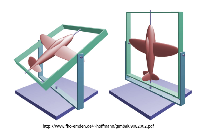
This problem is inherent to any decomposition into Euler angles, regardless of the chosen convention: there will always be a singular configuration. In animation, this manifests as erratic movements or “jumps” when the orientation passes in the vicinity of the singularity.
Another limitation of Euler angles concerns interpolation: linearly interpolating the three angles between two orientations indeed produces a rotation at every instant, but the path followed does not necessarily correspond to the most natural rotation trajectory (the shortest path on the orientation sphere). An object rotating from A to B may, with Euler angles, take a detour through intermediate, non-intuitive orientations.
The Euler’s rotation theorem (not to be confused with Euler angles) states that any rotation in 3D can be described by a unit axis \(\mathbf{n}\) (\(\|\mathbf{n}\| = 1\)) about which the rotation takes place, and an angle \(\theta\) that measures the amplitude of this rotation. This result is intuitive: any motion that leaves a fixed point (the origin) and preserves distances is necessarily a rotation about an axis passing through that point.
This representation is particularly natural for describing the rotation that brings a vector \(\mathbf{u}_1\) to a vector \(\mathbf{u}_2\) (both assumed unit vectors). The rotation axis is perpendicular to the plane formed by the two vectors, and the angle is the one that separates them:
Degenerate cases: this formula assumes that \(\mathbf{u}_1\) and \(\mathbf{u}_2\) are not collinear. If \(\mathbf{u}_1 = \mathbf{u}_2\) (parallel vectors), the rotation is the identity. If \(\mathbf{u}_1 = -\mathbf{u}_2\) (antiparallel vectors, \(\theta = \pi\)), the cross product is zero and the rotation axis is not uniquely determined — any vector perpendicular to \(\mathbf{u}_1\) is suitable. In practice, one chooses an arbitrary perpendicular axis (for example via a cross product with a reference vector).
The twist rotation around \(\mathbf{u}_2\) (rotation about the arrival axis after alignment) remains free and may be chosen arbitrarily — the pair \((\mathbf{n}, \theta)\) above corresponds to the choice of zero twist, i.e., to the rotation “the simplest” between the two vectors.
Advantages: concise representation (3 effective degrees of freedom, encoded in \(\mathbf{n}\) and \(\theta\), or equivalently in the vector \(\theta \mathbf{n} \in \mathbb{R}^3\)), geometrically meaningful parameters.
Disadvantages: composing two axis-angle rotations (i.e., finding the axis and angle of \(R_2 \circ R_1\) from \((\mathbf{n}_1, \theta_1)\) and \((\mathbf{n}_2, \theta_2)\)) does not admit a simple formula — one must go through matrices or quaternions. Direct interpolation in axis-angle is also less natural and less robust than via quaternions when the axes differ: interpolating the axis and the angle separately does not in general produce the shortest rotation path.
The central question is: given an axis \(\mathbf{n}\) and an angle \(\theta\), how can one compute the vector \(\mathbf{v}'\) obtained by rotating \(\mathbf{v}\)? The idea is to decompose \(\mathbf{v}\) into a component parallel to the axis (which does not move) and a perpendicular component (which rotates in the orthogonal plane):
\[ \mathbf{v}_\parallel = (\mathbf{v} \cdot \mathbf{n}) \, \mathbf{n}, \quad \mathbf{v}_\perp = \mathbf{v} - (\mathbf{v} \cdot \mathbf{n}) \, \mathbf{n} \] The parallel component \(\mathbf{v}_\parallel\) is the projection of \(\mathbf{v}\) onto the axis \(\mathbf{n}\). It is unchanged by the rotation (a vector aligned with the axis of rotation does not move). The perpendicular component \(\mathbf{v}_\perp\) lies in the plane orthogonal to \(\mathbf{n}\), and it is this one that rotates by an angle \(\theta\).
In this plane, there are two orthogonal vectors: \(\mathbf{v}_\perp\) and \(\mathbf{n} \times \mathbf{v}_\perp = \mathbf{n} \times \mathbf{v}\) (the latter is indeed perpendicular to both \(\mathbf{n}\) and \(\mathbf{v}_\perp\), and of the same magnitude as \(\mathbf{v}_\perp\)). The rotation of \(\mathbf{v}_\perp\) by an angle \(\theta\) in this plane gives:
\[ \mathbf{v}'_\perp = \cos(\theta) \, \mathbf{v}_\perp + \sin(\theta) \, \mathbf{n} \times \mathbf{v} \] By recombining \(\mathbf{v}' = \mathbf{v}_\parallel + \mathbf{v}'_\perp\) and substituting the expressions of \(\mathbf{v}_\parallel\) and \(\mathbf{v}_\perp\):
\[ \mathbf{v}' = \cos(\theta) \, \mathbf{v} + \sin(\theta) \, \mathbf{n} \times \mathbf{v} + (1 - \cos(\theta)) \, (\mathbf{v} \cdot \mathbf{n}) \, \mathbf{n} \] This is the Rodrigues’ formula.

We can verify the edge cases: for \(\theta = 0\), we obtain \(\mathbf{v}' = \mathbf{v}\) (no rotation); for \(\theta = \pi/2\), we obtain \(\mathbf{v}' = \sin(\pi/2) \, \mathbf{n} \times \mathbf{v} + (1 - \cos(\pi/2))(\mathbf{v} \cdot \mathbf{n}) \mathbf{n} = \mathbf{n} \times \mathbf{v} + (\mathbf{v} \cdot \mathbf{n}) \mathbf{n}\), i.e., a quarter turn of the perpendicular component (replacement by the orthogonal vector in the plane).
Rodrigues’ formula expresses \(\mathbf{v}'\) as a linear function of \(\mathbf{v}\) (each term — scalar product, cross product — is linear in \(\mathbf{v}\)). There exists therefore a matrix \(R\) such that \(\mathbf{v}' = R \, \mathbf{v}\). To obtain it, one rewrites each operation in matrix form.
The cross product \(\mathbf{n} \times \mathbf{v}\) corresponds to multiplication by the antisymmetric matrix:
\[ K = \begin{pmatrix} 0 & -n_z & n_y \\ n_z & 0 & -n_x \\ -n_y & n_x & 0 \end{pmatrix} \] such that \(K \, \mathbf{v} = \mathbf{n} \times \mathbf{v}\) for all \(\mathbf{v}\). The term \((\mathbf{v} \cdot \mathbf{n}) \, \mathbf{n}\) corresponds to the projection onto \(\mathbf{n}\), which is written \(\mathbf{n} \mathbf{n}^T \mathbf{v}\). Using the identity \(\mathbf{n} \mathbf{n}^T = I + K^2\) (valid when \(\|\mathbf{n}\| = 1\), since \(K^2 = \mathbf{n}\mathbf{n}^T - I\)), we can rewrite Rodrigues’ formula entirely in terms of \(K\) :
\[ R(\mathbf{n}, \theta) = \cos(\theta) \, I + \sin(\theta) \, K + (1 - \cos(\theta)) \, (I + K^2) \] which simplifies to:
\[ R(\mathbf{n}, \theta) = I + \sin(\theta) \, K + (1 - \cos(\theta)) \, K^2 \] By expanding the matrix products, one obtains explicitly:
\[ R = \begin{pmatrix} \cos\theta + n_x^2 (1 - \cos\theta) & n_x n_y (1 - \cos\theta) - n_z \sin\theta & n_x n_z (1 - \cos\theta) + n_y \sin\theta \\ n_x n_y (1 - \cos\theta) + n_z \sin\theta & \cos\theta + n_y^2 (1 - \cos\theta) & n_y n_z (1 - \cos\theta) - n_x \sin\theta \\ n_x n_z (1 - \cos\theta) - n_y \sin\theta & n_y n_z (1 - \cos\theta) + n_x \sin\theta & \cos\theta + n_z^2 (1 - \cos\theta) \end{pmatrix} \] We can verify that this matrix is indeed orthogonal and of determinant 1. For example, for \(\mathbf{n} = (0, 0, 1)\) (rotation about \(z\)), we obtain \(R_z(\theta)\) defined above.
The quaternions are a generalization of complex numbers to four dimensions. Where a complex number \(a + b \, \mathbf{i}\) has an imaginary unit \(\mathbf{i}\) (with \(\mathbf{i}^2 = -1\)), a quaternion has three imaginary units \(\mathbf{i}\), \(\mathbf{j}\), \(\mathbf{k}\):
\[ q = x \, \mathbf{i} + y \, \mathbf{j} + z \, \mathbf{k} + w \] With the short notation \(q = (x, y, z, w)\). The real part is \(w\), the imaginary part (or pure quaternion) is the triplet \((x, y, z)\). We also denote \(q = (\mathbf{s}, w)\) with \(\mathbf{s} = (x, y, z)\).
The imaginary bases satisfy the following multiplication rules:
\[ \mathbf{i}^2 = \mathbf{j}^2 = \mathbf{k}^2 = -1, \quad \mathbf{i}\mathbf{j} = \mathbf{k}, \quad \mathbf{j}\mathbf{k} = \mathbf{i}, \quad \mathbf{k}\mathbf{i} = \mathbf{j} \] et les produits dans l’ordre inverse changent de signe : \(\mathbf{j}\mathbf{i} = -\mathbf{k}\), \(\mathbf{k}\mathbf{j} = -\mathbf{i}\), \(\mathbf{i}\mathbf{k} = -\mathbf{j}\). On a aussi la relation \(\mathbf{i}\mathbf{j}\mathbf{k} = -1\). La ressemblance avec les règles du produit vectoriel n’est pas un hasard — le produit vectoriel peut se voir comme la partie imaginaire du produit de deux quaternions purs.
Note : ne pas confondre la notation \((x, y, z, w)\) d’un quaternion avec un vecteur 4D en coordonnées homogènes. Les quaternions vivent dans un espace algébrique muni de son propre produit, très différent de \(\mathbb{R}^4\).
The operations on quaternions are analogous to those of complex numbers:
The Product of two quaternions is computed by expanding the formal product and applying the multiplication rules of the bases. Denoting \(q_i = (\mathbf{s}_i, w_i)\) with \(\mathbf{s}_i = (x_i, y_i, z_i)\), we obtain the compact formula :
\[ q_1 \, q_2 = (\mathbf{s}_1 w_2 + \mathbf{s}_2 w_1 + \mathbf{s}_1 \times \mathbf{s}_2, \;\; w_1 w_2 - \mathbf{s}_1 \cdot \mathbf{s}_2) \] The imaginary part of the product combines a vector product (\(\mathbf{s}_1 \times \mathbf{s}_2\)) and scalar-vector cross terms, while the real part combines a scalar product and a product of real numbers. The product can also be written component by component:
\[ q_1 \, q_2 = \begin{pmatrix} x_1 w_2 + w_1 x_2 + y_1 z_2 - z_1 y_2 \\ y_1 w_2 + w_1 y_2 + z_1 x_2 - x_1 z_2 \\ z_1 w_2 + w_1 z_2 + x_1 y_2 - y_1 x_2 \\ w_1 w_2 - x_1 x_2 - y_1 y_2 - z_1 z_2 \end{pmatrix} \] The product of quaternions is associative (\(q_1 (q_2 q_3) = (q_1 q_2) q_3\)) but non-commutative (\(q_1 q_2 \neq q_2 q_1\)), as with matrix multiplication. The non-commutativity reflects the fact that 3D rotations do not commute: rotating first about the \(x\)-axis and then about the \(y\)-axis does not give the same result as the reverse order.
An important property of the product is that the conjugate of a product reverses order: \((q_1 q_2)^* = q_2^* q_1^*\) (as for the transpose of a product of matrices). Moreover, the product of two unit quaternions is unitary: \(\|q_1 q_2\| = \|q_1\| \cdot \|q_2\|\).
The link between quaternions and rotations rests on a construction that recalls complex numbers. In 2D, a unit complex number \(e^{i\theta} = \cos\theta + i \sin\theta\) represents a rotation by angle \(\theta\), and the rotation of a vector \(z\) is obtained by the product \(z' = e^{i\theta} \cdot z\). In 3D, the mechanism is similar but requires a “sandwich” product due to non-commutativity.
Let \(q = (\mathbf{s}, w)\) be a unit quaternion (\(\|q\| = 1\)), and \(\mathbf{v}\) a 3D vector associated with the pure quaternion \(q_v = (\mathbf{v}, 0)\) (zero real part). Then:
\[ q_{v'} = q \, q_v \, q^* = (\mathbf{v}', 0) \] is a pure quaternion (the real part is indeed zero — this is not obvious a priori), and \(\mathbf{v}'\) is the vector \(\mathbf{v}\) after rotation by angle \(2 \arccos(w)\) around the axis \(\mathbf{n} = \mathbf{s} / \|\mathbf{s}\|\).
The product “sandwich” \(q \, q_v \, q^*\) (multiplication on the left by \(q\) and on the right by \(q^*\)) is necessary for the result to be a pure quaternion: the simple product \(q \, q_v\) would have a nonzero real part and would not correspond to a 3D vector.
Demonstration. By expanding the triple product using the quaternion product formula:
\[ \mathcal{R}_q(\mathbf{v}) = q \, q_v \, q^* = ((w^2 - \|\mathbf{s}\|^2) \, \mathbf{v} + 2(\mathbf{s} \cdot \mathbf{v}) \, \mathbf{s} + 2w \, \mathbf{s} \times \mathbf{v}, \;\; 0) \] Since \(\|q\| = 1\), we can parameterize \(q = (\mathbf{n} \sin\phi, \cos\phi)\) with \(\|\mathbf{n}\| = 1\). By substituting \(\mathbf{s} = \mathbf{n} \sin\phi\) and \(w = \cos\phi\) :
\[ \mathcal{R}_q(\mathbf{v}) = \underbrace{(\cos^2\phi - \sin^2\phi)}_{\cos(2\phi)} \mathbf{v} + \underbrace{2 \sin^2\phi}_{1 - \cos(2\phi)} (\mathbf{n} \cdot \mathbf{v}) \, \mathbf{n} + \underbrace{2 \cos\phi \sin\phi}_{\sin(2\phi)} \, \mathbf{n} \times \mathbf{v} \] We recognize exactly the Rodrigues formula for the axis \(\mathbf{n}\) and the angle \(2\phi\). The factor 2 explains the half-angle in the correspondence:
The unit quaternion \(q = (\mathbf{n} \sin(\theta/2), \cos(\theta/2))\) represents the rotation by angle \(\theta\) about the axis \(\mathbf{n}\).
This half-angle has an important topological consequence: a rotation of \(2\pi\) (one full turn) corresponds to the quaternion \((\mathbf{n} \sin(\pi), \cos(\pi)) = (0, 0, 0, -1) = -1\), and an angle of \(4\pi\) is required to return to the quaternion \(+1\). The space of unit quaternions thus constitutes a double cover of \(SO(3)\): two quaternions \(+q\) and \(-q\) represent the same rotation (we will revisit this in the section on interpolation).
Let two rotations associated with unit quaternions \(q_1\) and \(q_2\). The product \(q_1 \, q_2\) represents the composition \(R_1 \circ R_2\).
The demonstration is straightforward:
\[ \mathcal{R}_{q_1 q_2}(\mathbf{v}) = (q_1 q_2) \, \mathbf{v} \, (q_1 q_2)^* = q_1 (q_2 \, \mathbf{v} \, q_2^*) q_1^* = q_1 \, \mathcal{R}_{q_2}(\mathbf{v}) \, q_1^* = \mathcal{R}_{q_1} \circ \mathcal{R}_{q_2}(\mathbf{v}) \] by using the property \((q_1 q_2)^* = q_2^* q_1^*\).
The unit quaternion \(q = (x, y, z, w)\) corresponds to the rotation matrix:
\[ R = \begin{pmatrix} 1 - 2(y^2 + z^2) & 2(xy - wz) & 2(xz + wy) \\ 2(xy + wz) & 1 - 2(x^2 + z^2) & 2(yz - wx) \\ 2(xz - wy) & 2(yz + wx) & 1 - 2(x^2 + y^2) \end{pmatrix} \] Conversely, from a rotation matrix \(M\), one can extract the corresponding quaternion. When the trace of \(M\) is positive (\(1 + M_{xx} + M_{yy} + M_{zz} > 0\)), we use:
\[ q = \left(\frac{M_{zy} - M_{yz}}{2r}, \; \frac{M_{xz} - M_{zx}}{2r}, \; \frac{M_{yx} - M_{xy}}{2r}, \; \frac{r}{2}\right), \quad r = \sqrt{1 + M_{xx} + M_{yy} + M_{zz}} \] When the trace is near zero or negative (which occurs for rotations close to \(\pi\)), this formula becomes numerically unstable (\(r \to 0\)). In practice, a case-based version is used that selects the dominant diagonal component to avoid divisions by values close to zero.
| Representation | Advantages | Disadvantages |
|---|---|---|
| Matrix | Direct computation, straightforward composition | Implicit parameters (9 coefficients for 3 DOF) |
| Euler angles | Understandable parameters, direct interaction | Gimbal lock, unsuitable interpolation |
| Axis-angle | Concise, intuitive | No straightforward composition |
| Quaternion | Composition, interpolation, no gimbal lock | Less intuitive components |
The following table provides a comparative indication of the cost of common operations according to the representation ; the actual performances depend on the implementation and hardware :
| Operation | Matrix | Quaternion |
|---|---|---|
| Storage | 9 floats | 4 floats |
| Rotation of a vector | fast | moderate |
| Composition | moderate | fast |
| Inversion | negligible (transpose) | negligible (conjugate) |
| Interpolation | costly (matrix exponential/log) | fast (SLERP) |
Rotating a vector with a matrix is faster, but composing rotations and interpolation are more efficient with quaternions. In practice, orientations are stored and interpolated in quaternions, then converted to matrices at render time (the GPU expects matrices).
Rotation interpolation occurs as soon as we want to animate an orientation: a transition between two poses of a character, progressive rotation of the camera, interpolation between the keyframes of an animation. Given two rotations \(r_1\) and \(r_2\), we seek a rotation \(r(t)\) varying continuously with \(t \in [0, 1]\) such that \(r(0) = r_1\) and \(r(1) = r_2\).
The difficulty is that rotations do not live in a vector space: the intermediate result must be a valid rotation at every instant \(t\), without parasitic scaling or shearing. Not all representations lend themselves equally to interpolation:
The simplest approach is to linearly interpolate the quaternions in \(\mathbb{R}^4\), and then renormalize the result to return to the unit sphere:
\[ q(t) = \frac{(1 - t) \, q_1 + t \, q_2}{\|(1 - t) \, q_1 + t \, q_2\|} \] Geometrically, the linear combination \((1-t) q_1 + t q_2\) produces a point inside the sphere (on the chord connecting \(q_1\) to \(q_2\)), and the normalization reprojects it onto the sphere. The resulting path on the sphere indeed follows the great circle (the shortest path), but the speed along this path is not constant: the parameterization is faster at the ends (\(t\) close to 0 or 1) and slower in the middle. Indeed, radial reprojection “concentrates” the points toward the middle of the arc.

LERP can be generalized to parametric curves (quaternion splines, etc.), which makes it a useful tool for animations with more than two key-frames. On the other hand, the non-constant angular velocity can pose problems for applications requiring smooth motion.
To obtain a constant angular velocity (the rotation progresses uniformly with \(t\)), we use the spherical linear interpolation (SLERP). The idea is to interpolate directly on the sphere rather than going through a chord and then reproject.
Let \(\Omega\) be the angle between \(q_1\) and \(q_2\) in 4D space, defined by \(\cos(\Omega) = q_1 \cdot q_2\) (dot product of the 4 components):
\[
q(t) = \frac{\sin((1 - t) \, \Omega)}{\sin(\Omega)} \, q_1 +
\frac{\sin(t \, \Omega)}{\sin(\Omega)} \, q_2
\] 
Demonstration. We construct an orthonormal frame in the plane \((q_1, q_2)\), with \(q_1\) as the first vector and \(q_1^\perp = \frac{q_2 - \cos(\Omega) \, q_1}{\sin(\Omega)}\) as the second. The vector at angle \(\theta = \Omega \, t\) from \(q_1\) is written \(q(t) = q_1 \cos(\Omega t) + q_1^\perp \sin(\Omega t)\). By substituting \(q_1^\perp\) and using the identity \(\sin(\Omega) \cos(\Omega t) - \cos(\Omega) \sin(\Omega t) = \sin((1-t)\Omega)\), we recover the SLERP formula. We verify that \(q(0) = q_1\), \(q(1) = q_2\), and \(\|q(t)\| = 1\) for all \(t\).
Advantages of SLERP : shortest path on the sphere, constant angular velocity, the result is always of unit length.
Disadvantage : does not generalize directly to interpolation between more than two quaternions. For animations with \(N\) key-frames, one uses derivative-based methods, often based on the normalized LERP (nLERP) which, although not having a constant angular velocity, lends itself more readily to the construction of splines.
Degenerate case : when \(\Omega\) is very small (\(q_1 \approx q_2\)), the denominator \(\sin(\Omega)\) tends to 0 and the formula becomes numerically unstable. In practice, we switch to the LERP (with renormalization) when \(\Omega\) is below a threshold (typically \(10^{-4}\)).
As mentioned above, the quaternions \(+q\) and \(-q\) represent the same rotation (since \(\mathbf{n} \to -\mathbf{n}\) and \(\theta \to 2\pi - \theta\), the sandwich product remains identical). However, on the sphere \(S^3\), \(+q\) and \(-q\) are two antipodal points, and they correspond to different interpolation paths.
The SLERP interpolation between \(q_1\) and \(q_2\) follows the shortest arc of a great circle on the sphere. But there are two possible arcs between \(q_1\) and \(q_2\) (the short and the long), and the arc between \(q_1\) and \(-q_2\) is the complement of the one between \(q_1\) and \(q_2\). Concretely :
In practice, if one forgets this check, the object may rotate “through the long path” — a rotation of 350° instead of 10° — which yields visually aberrant motion. We fix this by inverting \(q_2\) when necessary:
if (dot(q1, q2) < 0)
    q2 = -q2;

q_t = slerp(q1, q2, t);Let’s show that constant speed on the sphere of quaternions implies a constant angular velocity in 3D.
Let \(q(t)\) be a unit quaternion depending on time, and \(R(t)\) the associated 3D rotation. The angular velocity \(\boldsymbol{\omega}(t) \in \mathbb{R}^3\) is defined by the relation \(\dot{R} = [\boldsymbol{\omega}]_\times R\), where \([\boldsymbol{\omega}]_\times\) is the skew-symmetric matrix associated with the cross product by \(\boldsymbol{\omega}\). In terms of quaternions, this relation translates to :
\[ \dot{q} = \frac{1}{2} \, \boldsymbol{\omega}_q \, q \] where \(\boldsymbol{\omega}_q = ({\omega_x}, {\omega_y}, {\omega_z}, 0)\) is the pure quaternion associated with the vector \(\boldsymbol{\omega}\). By inverting this relation (\(q\) is unitary, hence \(q^{-1} = q^*\)) :
\[ \boldsymbol{\omega}_q = 2 \, \dot{q} \, q^* \] The norm of the angular velocity is therefore \(\|\boldsymbol{\omega}\| = 2 \|\dot{q}\|\) (since \(\|q^*\| = 1\) and quaternion multiplication preserves norms). This factor 2 arises from the half-angle in the quaternion-rotation correspondence.
For SLERP, \(q(t)\) traces a great-circle arc on \(S^3\) at a constant speed \(\|\dot{q}\|\) (by construction of spherical linear interpolation). The relation \(\|\boldsymbol{\omega}\| = 2\|\dot{q}\|\) then shows that the 3D angular velocity is also constant. Concretely, the geodesic distance \(\Omega\) on \(S^3\) between \(q_1\) and \(q_2\) is related to the 3D rotation angle \(\theta\) between \(R_1\) and \(R_2\) by \(\Omega = \theta / 2\), and the SLERP traverses this distance uniformly.
In practice, a 3D object is characterized by an orientation \(r\) (rotation) and a position \(\mathbf{p}\) (translation). To interpolate between two configurations \((r_1, \mathbf{p}_1)\) and \((r_2, \mathbf{p}_2)\) — for example to animate an object that moves while rotating — we interpolate the two components separately:
The combination of the two yields a rigid motion (no deformation) that varies smoothly between the two configurations. This is the standard interpolation used in animation engines for the position and orientation keyframes.
When the transformations include scaling or deformation (shearing) in addition to rotation and translation, a simple interpolation SLERP + linear is no longer sufficient. It is necessary to first separate the different components of the transformation and interpolate each of them appropriately.
The key mathematical tool is the polar decomposition: every invertible 3 × 3 matrix can be decomposed as \(M = R \, D\), where \(R\) is a rotation matrix (\(R \in SO(3)\) ) and \(D\) is a symmetric positive semi-definite matrix (which encodes the scaling and the shearing). This decomposition is the matrix analogue of writing a complex number in polar form \(z = r \, e^{i\theta}\). It can be computed by SVD (\(M = U \Sigma V^T\), then \(R = U V^T\) and \(D = V \Sigma V^T\)) or by the iterative scheme \(R_{i+1} = \frac{1}{2}(R_i + (R_i^{-1})^T)\) starting from \(R_0 = M\).
Linear interpolation of \(M\) without prior decomposition produces artifacts: an object that should rotate smoothly deforms temporarily and then returns to its initial shape. The polar decomposition allows interpolating each component with the appropriate method.
The complete algorithm for interpolating between two general \(4 \times 4\) matrices \(M_1\) and \(M_2\) is:
Let an affine transformation \(M\) be applied to the positions of an object: \(\mathbf{p}' = M \mathbf{p}\). Tangent vectors to the surface, defined as differences of neighboring positions, transform by the same matrix: \(\mathbf{t}' = M \mathbf{t}\). The question is to determine how the normals \(\mathbf{n}\) transform under the action of \(M\).
For a rotation \(R\), the normal transforms as \(\mathbf{n}' = R \mathbf{n}\): orthogonality is preserved because \(R\) preserves angles. For a uniform scaling \(sI\), the direction of the normal remains unchanged (only its magnitude is affected, corrected by renormalization). In these two cases, applying \(M\) directly to the normals yields a correct result (up to renormalization).
The problem arises in the presence of non-uniform scaling or shear. Consider a horizontal plane with a vertical normal \(\mathbf{n} = (0, 1, 0)\), and apply a horizontal stretch \(S = \text{diag}(2, 1, 1)\) (doubling the \(x\) coordinate). The surface stretches horizontally, but the normal remains vertical — it should not change. Now, \(S \mathbf{n} = (0, 1, 0) = \mathbf{n}\), which is correct in this case. Now, take a plane inclined at 45° with \(\mathbf{n} = (1, 1, 0)/\sqrt{2}\). After the horizontal stretch, the plane is “flattened” and its normal should tilt toward the vertical. But \(S \mathbf{n} = (2, 1, 0)/\sqrt{5}\), which tilts in the opposite direction toward the horizontal — the result is false. The normal transformed by \(M\) is no longer perpendicular to the transformed surface.
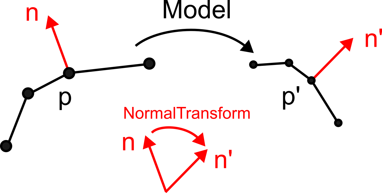
The fundamental property of a normal is its orthogonality to the tangents of the surface. Let \(\mathbf{t}\) be a tangent vector to the surface at a point \(\mathbf{p}\). Before transformation: \(\mathbf{n} \cdot \mathbf{t} = 0\). After transformation, the tangents transform by \(\mathbf{t}' = M \mathbf{t}\), and we seek the matrix \(N\) such that the transformed normals \(\mathbf{n}' = N \mathbf{n}\) satisfy \(\mathbf{n}' \cdot \mathbf{t}' = 0\) for every tangent \(\mathbf{t}\).
By expanding the orthogonality condition after transformation:
\[ (N \mathbf{n})^T (M \mathbf{t}) = \mathbf{n}^T N^T M \mathbf{t} = 0 \] We know that \(\mathbf{n}^T \mathbf{t} = 0\). A sufficient (and the simplest) condition for \(\mathbf{n}^T (N^T M) \mathbf{t} = 0\) for all \(\mathbf{t}\) orthogonal to \(\mathbf{n}\) is that \(N^T M = I\), that is:
\[ N = (M^{-1})^T \] The normal transformation matrix is the transpose of the inverse of the transformation matrix of positions (often denoted \(M^{-T}\)).
In GLSL, we work with the 3 × 3 submatrix of the Model matrix (which contains the rotation and the scaling, without translation — normals are directions, not positions):
mat3 normalMatrix = transpose(inverse(mat3(Model)));
vec3 n = normalize(normalMatrix * vertex_normal);
The call mat3(Model) extracts the top-left \(3 \times 3\) submatrix. The final
renormalization is necessary because \((M^{-1})^T\) does not preserve the norm in
general.
When \(M\) is a pure rotation (or a rigid transformation: rotation + translation), we have \(M^{-1} = M^T\) (because \(R^{-1} = R^T\) for rotations), hence \(N = (M^{-1})^T = M\). The normal transformation coincides with that of positions: normals transform by the same matrix, without special treatment.
When \(M\) contains a uniform scaling \(s\) in addition to the rotation (\(M = sR\)), we obtain \(N = (s^{-1} R^{-1})^T = s^{-1} R\). The factor \(s^{-1}\) changes the magnitude of the normal, but not its direction. After renormalization, the result is identical to \(R \mathbf{n}\).
The non-trivial case appears only in the presence of non-uniform scaling (factors different along the axes) or of shearing. It is in these cases that the use of \((M^{-1})^T\) is indispensable to obtain correct lighting.
Performance note: the calculation of
transpose(inverse(Model)) at each fragment is costly. In
practice, this matrix is pre-calculated on the CPU side and sent to the
shader as a uniform, just like the Model matrix itself.
The order in which transformations are applied is fundamental and constitutes a common source of errors in computer graphics programming. For a rotation \(R\) and a translation \(\mathbf{t}\), one generally has:
\[ T \, R \neq R \, T \] Transformation matrices (in homogeneous coordinates \(4 \times 4\)) are applied from right to left: in the product \(M \, \mathbf{p} = (A \, B) \, \mathbf{p}\), it is \(B\) that is applied first to the point \(\mathbf{p}\), then \(A\) to the result. This order “inverted” relative to reading is a standard mathematical convention, but one must get used to it.
Let’s detail the two cases on a concrete example.
Case 1 : \(M_1 = T \, R\) (rotation first, then translation)
\[ M_1 = \begin{pmatrix} I & \mathbf{t} \\ 0 & 1 \end{pmatrix} \begin{pmatrix} R & 0 \\ 0 & 1 \end{pmatrix} = \begin{pmatrix} R & \mathbf{t} \\ 0 & 1 \end{pmatrix} \] The object is first rotated about the origin (its vertices are multiplied by \(R\)), then the set is translated by \(\mathbf{t}\). The result is a rotated object, whose center is at the position \(\mathbf{t}\). This is the typical case of the placement of an object in the scene: we orient it first (rotation), then position it (translation).
Case 2 : \(M_2 = R \, T\) (first translation, then rotation)
\[ M_2 = \begin{pmatrix} R & 0 \\ 0 & 1 \end{pmatrix} \begin{pmatrix} I & \mathbf{t} \\ 0 & 1 \end{pmatrix} = \begin{pmatrix} R & R \, \mathbf{t} \\ 0 & 1 \end{pmatrix} \] The object is first translated by \(\mathbf{t}\) (away from the origin), then the whole set is rotated about the origin. As the rotation is applied about the origin, the object traces an arc of a circle. The effective translation is no longer \(\mathbf{t}\) but \(R \, \mathbf{t}\): the translation vector itself has been rotated. This is the typical case of the orbit: an object away from the origin that revolves around it.


À gauche : $M_1 = T \, R$ (rotation puis translation). À droite : $M_2 = R \, T$ (translation puis rotation autour de l'origine).
The difference between the two cases is striking: \(M_1\) produces an object rotated in place and then translated, while \(M_2\) produces an object that orbits around the origin. The confusion between these two cases is one of the most common errors in 3D programming.
Warning: some libraries (legacy OpenGL in
fixed-pipeline mode, Three.js) use a matrix multiplication convention
that is transposed relative to the standard
mathematical convention. In these libraries, the transformations are
applied from left to right in the code. For example, in legacy OpenGL,
the code glTranslate(); glRotate(); applies first the
translation, then the rotation — which corresponds to \(M_2 = R \, T\) in our convention. You
should consult the documentation of each library to know which
convention is used.
Rotations expressed by matrices \(R\) are always performed around the origin. To apply a rotation around an arbitrary point \(\mathbf{p}_0\), the classic scheme consists of three steps: (1) translate to bring \(\mathbf{p}_0\) to the origin, (2) perform the rotation, (3) translate back to restore \(\mathbf{p}_0\) to its position:
\[ M = T(\mathbf{p}_0) \, R \, T(-\mathbf{p}_0) \] By expanding the product of the three \(4 \times 4\) matrices:
\[ M = \begin{pmatrix} I & \mathbf{p}_0 \\ 0 & 1 \end{pmatrix} \begin{pmatrix} R & 0 \\ 0 & 1 \end{pmatrix} \begin{pmatrix} I & -\mathbf{p}_0 \\ 0 & 1 \end{pmatrix} = \begin{pmatrix} R & \mathbf{p}_0 - R \, \mathbf{p}_0 \\ 0 & 1 \end{pmatrix} \] We can verify that \(M \, \mathbf{p}_0 = R \, \mathbf{p}_0 + \mathbf{p}_0 - R \, \mathbf{p}_0 = \mathbf{p}_0\) : the point \(\mathbf{p}_0\) is indeed fixed, as expected.
This scheme is ubiquitous in practice. For example, to rotate a mesh around its barycenter \(\bar{\mathbf{p}} = \frac{1}{N} \sum_{i=1}^{N} \mathbf{p}_i\), one uses \(M = T(\bar{\mathbf{p}}) \, R \, T(-\bar{\mathbf{p}})\). To rotate an articulated arm around the shoulder, one first translates the shoulder to the origin, applies the rotation, and then translates back. This pattern “translate-rotate-untranslate” appears at every articulation of an animation skeleton.
An affine transformation parameterized by a uniform scaling \(s\), a rotation \(R\) and a translation \(\mathbf{t}\) is written in the form of a block matrix \(4 \times 4\):
\[ M = T \, R \, S = \begin{pmatrix} s \, R & \mathbf{t} \\ 0 & 1 \end{pmatrix} \] Its inverse is \((AB)^{-1} = B^{-1} A^{-1}\), therefore \(M^{-1} = S^{-1} \, R^{-1} \, T^{-1}\). Expanding:
\[ M^{-1} = \begin{pmatrix} \frac{1}{s} R^T & -\frac{1}{s} R^T \mathbf{t} \\ 0 & 1 \end{pmatrix} \] Each component simply inverts: the translation by \(-\mathbf{t}\), the rotation by \(R^T\), the scale by \(1/s\). However, these inverses must be applied in the reverse order to that of the original composition, which explains the term \(-\frac{1}{s} R^T \mathbf{t}\) (and not simply \(-\mathbf{t}\)) in the translation block.
In computer graphics, the objects of a scene are almost never independent of one another. A character has arms attached to the torso, a vehicle has wheels attached to the chassis, a solar system has moons orbiting around planets that orbit around a star. In each of these cases, the movement of a child object is defined relative to a parent object: the hand moves relative to the forearm, which moves relative to the arm, which moves relative to the torso.
This hierarchical organization is formalized by a frame hierarchy (or frame hierarchy). Each object possesses a local transformation \(M_{\text{local}}\) that describes its position and its orientation relative to its parent. The transformation global (or world transform) that places the object in the world frame is obtained by composing all the local transformations from the root of the hierarchy:
\[ M_{\text{global}} = M_{\text{parent}}^{\text{global}} \; M_{\text{local}} \] By developing recursively:
\[ M_{\text{global}}^{(i)} = M_{\text{local}}^{(0)} \; M_{\text{local}}^{(1)} \; \ldots \; M_{\text{local}}^{(i)} \] where \(M_{\text{local}}^{(0)}\) is the transformation of the root (often the identity), \(M_{\text{local}}^{(1)}\) the transformation of its child, etc. The matrices are composed from left to right in the hierarchy, which corresponds to applying from right to left on the points: a point \(\mathbf{p}\) of the object \((i)\), expressed in the local frame of \((i)\), is transformed first by \(M_{\text{local}}^{(i)}\), then by \(M_{\text{local}}^{(i-1)}\), etc.
Each local transformation is a rigid transformation (rotation + translation), represented in homogeneous coordinates by a \(4 \times 4\) matrix of the form:
\[ M = \begin{pmatrix} R & \mathbf{t} \\ 0 & 1 \end{pmatrix} \] where \(R \in SO(3)\) is the rotation matrix \(3 \times 3\) and \(\mathbf{t} \in \mathbb{R}^3\) the translation vector. The composition of two such transformations is computed blockwise:
\[ M_{\text{global}} = M_{\text{parent}} \; M_{\text{local}} = \begin{pmatrix} R_p & \mathbf{t}_p \\ 0 & 1 \end{pmatrix} \begin{pmatrix} R_l & \mathbf{t}_l \\ 0 & 1 \end{pmatrix} = \begin{pmatrix} R_p R_l & R_p \mathbf{t}_l + \mathbf{t}_p \\ 0 & 1 \end{pmatrix} \] The global rotation is therefore the product of the rotations \(R_g = R_p R_l\), and the global translation is \(\mathbf{t}_g = R_p \mathbf{t}_l + \mathbf{t}_p\). The term \(R_p \mathbf{t}_l\) expresses the fact that the local translation of the child is expressed in the parent frame — it must be rotated by the parent’s rotation before being added to the parent’s translation.
If one includes a uniform scaling \(s\) (which is common in scene graphs), the local transformation takes the form :
\[ M = \begin{pmatrix} s R & \mathbf{t} \\ 0 & 1 \end{pmatrix} \] and the composition yields:
\[ M_{\text{global}} = \begin{pmatrix} s_p R_p \; s_l R_l & s_p R_p \mathbf{t}_l + \mathbf{t}_p \\ 0 & 1 \end{pmatrix} = \begin{pmatrix} s_p s_l \; R_p R_l & s_p R_p \mathbf{t}_l + \mathbf{t}_p \\ 0 & 1 \end{pmatrix} \] Global scaling is the product \(s_g = s_p \, s_l\), the global rotation remains \(R_g = R_p R_l\), and the local translation is both rotated and scaled by the parent: \(\mathbf{t}_g = s_p R_p \mathbf{t}_l + \mathbf{t}_p\).
The above formulas apply to rigid transformations and uniform scaling. In the presence of non-uniform scaling or shear, the decomposition into rotation / translation / scale becomes more delicate, and hierarchical propagation no longer reduces to these simple formulas.
Fundamental property : when you modify the local transformation of a node, all of its descendants are automatically affected. If the torso rotates by 30°, the arms, forearms, hands and fingers follow the movement without the need to modify their local transformations. This is exactly the expected behavior: rotating the torso of a character naturally drives the entire upper body.
An articulated object is a special case of a frame hierarchy in which the nodes are joints (articulations) connected by rigid segments. The skeleton of a character is the most common example: each articulation (shoulder, elbow, wrist, hip, knee, ankle…) defines a local frame, and the local transformation of each articulation is typically a rotation (the bones do not deform; they pivot around the joints).
Consider the example of a two-segment articulated arm (upper arm + forearm) in the plane:
The global transformation of the elbow is:
\[ M_{\text{coude}} = T(\mathbf{p}_0) \; R(\alpha) \; T(L_1, 0, 0) \] The global transformation of the hand is:
\[ M_{\text{main}} = \underbrace{T(\mathbf{p}_0) \; R(\alpha) \; T(L_1, 0, 0)}_{M_{\text{coude}}} \; R(\beta) \; T(L_2, 0, 0) \] We observe the repeating pattern: at each articulation, we compose a local rotation (the articulation angle) followed by a translation along the segment (the length of the bone). To animate the arm, it suffices to vary the angles α(t) and β(t) over time — the global positions of all points are updated automatically by propagation through the chain.
This model generalizes directly to 3D: each articulation has a 3D rotation (typically stored as a quaternion for interpolation), and the local transformation includes the translation along the bone.
At the scale of an entire scene, the hierarchy of frames generalizes into a scene graph (scene graph). It is a tree structure (or more generally a DAG — directed acyclic graph) in which each node carries a local transformation and may contain geometry, light sources, cameras, or other child nodes.
A typical scene graph might have the following structure:
Scène (racine)
├── Terrain
├── Personnage
│   ├── Torse
│   │   ├── Bras_gauche
│   │   │   ├── Avant_bras_gauche
│   │   │   │   └── Main_gauche
│   │   │   ...
│   │   └── Tête
│   └── Jambe_gauche
│       └── Pied_gauche
├── Véhicule
│   ├── Châssis
│   ├── Roue_avant_gauche
│   ├── Roue_avant_droite
│   ...
└── Caméra
The update of global coordinates consists of traversing the nodes in hierarchical order (parents before children) and composing each local transformation with the parent’s global transformation.
In practice, an efficient implementation represents each node by its geometry, an identifier, the identifier of its parent, and its local transformation:
struct node {
    mesh geometry;              // géométrie associée au nœud
    std::string name;           // identifiant du nœud
    std::string name_parent;    // identifiant du parent
    mat4 transform_local;       // transformation par rapport au parent
    mat4 transform_global;      // transformation dans le repère monde
};
Nodes are stored in an ordered array such that every parent appears before its children, and a name \(\to\) index mapping table allows fast lookup of a node:
struct hierarchy {
    std::vector<node> elements;        // parents avant enfants
    std::map<std::string, int> index;  // accès rapide par nom
};
The propagation of the transformations is then reduced to a simple linear traversal of the array:
int const N = elements.size();
for (int k = 0; k < N; ++k) {
    auto& element = elements[k];

    if (element est un nœud racine) {
        // La transformation globale est la transformation locale
        element.transform_global = element.transform_local;
    }
    else {
        // Composition avec la transformation globale du parent
        auto const& local  = element.transform_local;
        auto const& global_parent
            = elements[index_parent].transform_global;
        element.transform_global = global_parent * local;
    }
}
The algorithm is O(N): each node is visited only once, and the parent’s global transform is already computed thanks to the order of the array. To animate the hierarchy, simply modify the local transformations of the desired nodes, then re-run this propagation before rendering.
Advantages of the scene graph :
The matrix View transforms the coordinates of the world space (scene’s global frame) to coordinates of the view space (frame attached to the camera, in which the camera is at the origin and looks in the direction \(-z\)). This transformation is necessary because the rendering pipeline works in the camera space for perspective projection (see the chapter on the rendering pipeline).
The camera is defined in the world space by its position \(\mathbf{eye}\) and its local frame consisting of three orthonormal vectors: \(\mathbf{right}\) (right direction), \(\mathbf{up}\) (up direction) and \(\mathbf{back}\) (direction opposite to the viewing direction). The camera matrix \(\text{Cam}\) is the matrix \(4 \times 4\) that transforms coordinates of the view space into coordinates of the world space — it is the matrix whose columns are the vectors of the camera frame expressed in the world frame:
\[ \text{Cam} = \begin{pmatrix} | & | & | & | \\ \mathbf{right} & \mathbf{up} & \mathbf{back} & \mathbf{eye} \\ | & | & | & | \\ 0 & 0 & 0 & 1 \end{pmatrix} = \begin{pmatrix} O & \mathbf{eye} \\ 0 & 1 \end{pmatrix} \] where \(O = (\mathbf{right} \;|\; \mathbf{up} \;|\; \mathbf{back})\) is the 3×3 orientation matrix. The view matrix is its inverse (it performs the transformation in the opposite direction: world \(\to\) view) :
\[ \text{View} = \text{Cam}^{-1} = \begin{pmatrix} O^T & -O^T \, \mathbf{eye} \\ 0 & 1 \end{pmatrix} \] The inverse is computed simply because \(\text{Cam}\) is a rigid transformation (rotation + translation): the rotation is inverted by transposition (\(O^{-1} = O^T\)) and the translation is inverted as \(-O^T \mathbf{eye}\). We can verify that \(\text{View} \times \mathbf{eye} = (0, 0, 0, 1)\): the camera’s position is indeed at the origin in the view space.
In practice, the view matrix is often constructed via a function
lookAt(eye, center, up_hint) which computes the camera
frame from the camera position (\(\mathbf{eye}\)), the target point (\(\mathbf{center}\)) and an approximate “up”
vector (\(\mathbf{up_hint}\), typically
the y-axis). The algorithm is :
An easy approach to control the camera in a 3D viewer consists of parameterizing its position in spherical coordinates \((\theta, \varphi, r)\) around a central point \(\mathbf{center}\). The camera orbits on a sphere of radius \(r\), and the user controls the latitude \(\varphi\) and longitude \(\theta\) with the mouse, the radius \(r\) with the scroll wheel.
The position of the camera is then:
\[
\mathbf{eye} = \mathbf{center} + r \, (\cos\varphi \cos\theta, \;
\sin\varphi, \; \cos\varphi \sin\theta)
\] and the view matrix is reconstructed at each frame via
lookAt(eye, center, up).
Advantages: simple implementation, convenient for orbiting around a structure with a natural orientation (building, standing character).
Disadvantages: there is a missing degree of freedom
— the camera orientation is entirely determined by its position on the
sphere, with no possibility of twist rotation (roll around the viewing
axis). Moreover, at the poles (\(\varphi = \pm
\pi/2\)), the vector \(\mathbf{up\_hint}\) becomes parallel to the
viewing direction, which causes degeneracy (the cross product in
lookAt yields a zero vector). Finally, if the observed
object has an initial orientation that does not match the convention “up
= \(y\)”, mouse movements no longer
correspond to the expected rotations.
The ArcBall (or Trackball), proposed by K. Shoemake (ARCBALL: A User Interface for Specifying Three-Dimensional Orientation Using a Mouse, Graphics Interface, 1992), offers three degrees of freedom for the orientation of the camera and overcomes the limitations of spherical coordinates.
The idea is as follows: one imagines a virtual sphere (the trackball) centered in the middle of the screen. When the user clicks and drags the mouse, the two cursor positions (the start and end of the drag) are projected onto this sphere, producing two three-dimensional points. The rotation that brings the first point to the second defines the rotation to apply to the camera (or to the object).
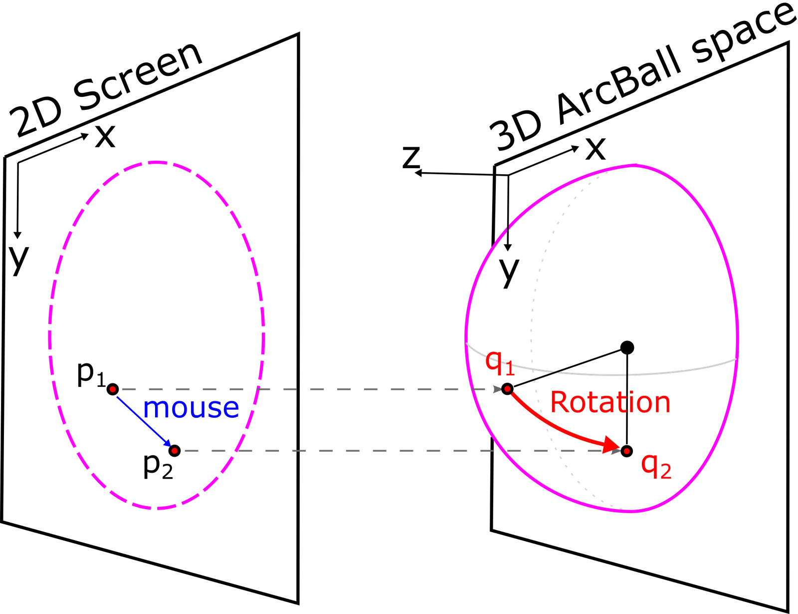
The algorithm is as follows. Let \(\mathbf{p}_1 = (p_{1x}, p_{1y})\) and \(\mathbf{p}_2 = (p_{2x}, p_{2y})\) be two cursor positions in normalized screen coordinates (in \([-1, 1]\)):
The projection onto the trackball uses a sphere for positions near the center and a hyperbolic extension for distant positions (to cover the entire screen):
\[ \text{ProjectionArcBall}(\mathbf{p}) = \begin{cases} (\mathbf{p}, \sqrt{1 - d^2}) & \text{si } d < 1/\sqrt{2} \quad \text{(sphère)} \\ (\mathbf{p}, 1/(2d)) & \text{sinon} \quad \text{(hyperbole)} \end{cases} \] with \(d = \|\mathbf{p}\|\). The transition between the sphere and the hyperbola occurs at \(d = 1/\sqrt{2}\), the point at which the two functions (\(\sqrt{1-d^2}\) and \(1/(2d)\)) coincide in value and derivative, ensuring a smooth transition.
Advantages: natural rotation around forms, no privileged axis (unlike spherical coordinates which singularize the poles), invariant behavior regardless of the initial orientation of the object.
Disadvantages: the rotation obtained is less “neat” than independent control of each axis (pitch, yaw, roll) — which can hinder very precise camera movements. Moreover, rapid back-and-forth mouse movements cause a slight drift (orientation drift), because the discretization of the cursor positions introduces small cumulative errors.
The traditional approach to animation consists in manually defining the trajectory of objects — either by keyframes (the animator fixes the position and orientation at certain moments, then the software interpolates between these poses), or by scripted procedural motions (for example, rotating a wheel at a constant speed). This approach works very well as long as the movement remains predictable and the animator can mentally conceive its form.
But many phenomena escape this direct control. A cape that wrinkles as the wind blows, a fluid that flows, a pile of marbles that collapses, hair that follows the movement of a character: in all these cases, the dynamics itself is the desired effect. The final shape is not known in advance; it emerges from the interactions among numerous elements subjected to forces. Attempting to manually specify the position of every fold or every drop would be both tedious and unconvincing.
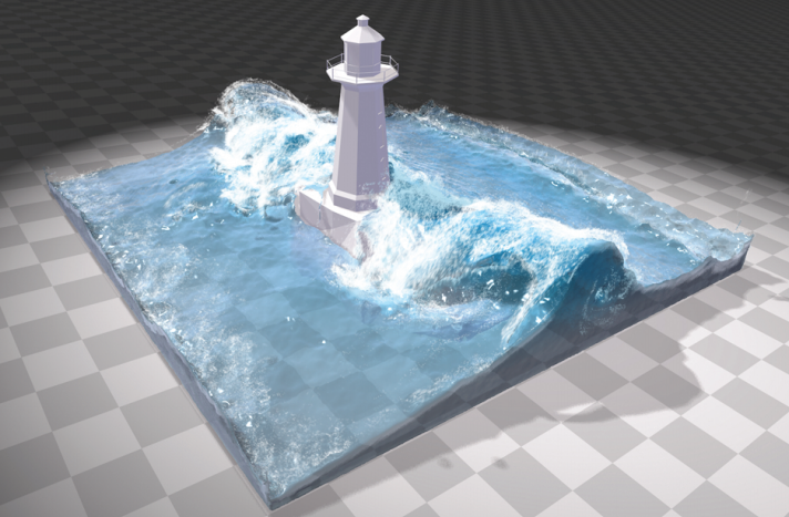
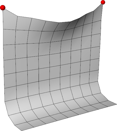
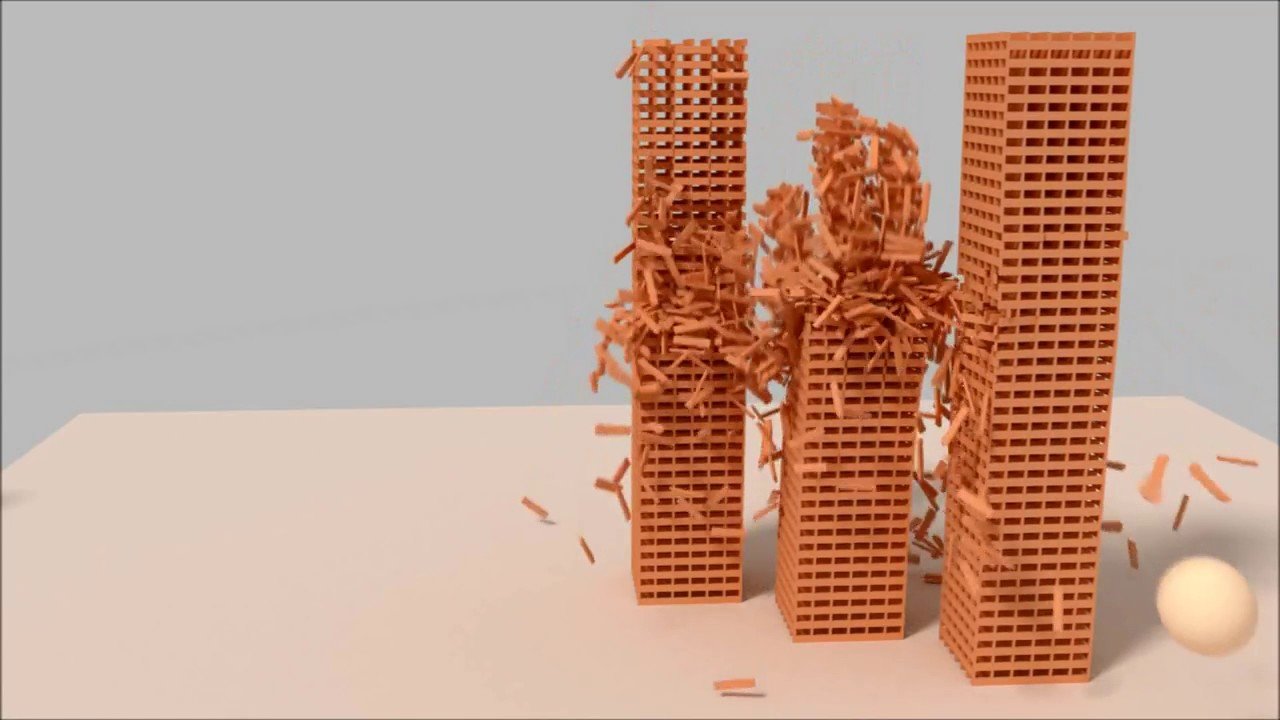
Trois exemples de phénomènes nécessitant une simulation physique : fluides, tissu, dynamique d'objets rigides multiples.
It is in these situations that the physical simulation becomes indispensable: we entrust the calculation with the task of generating motion, starting from a description of the system and its evolution laws. The result is obtained not by drawing the trajectory, but by deriving it from a mathematical model.
Any physical simulation, regardless of the phenomenon being modeled, follows the same three-step approach.
Description of the system. We first choose the parameters that characterize the state of the system at a given instant: positions, velocities, orientations, temperatures, densities, etc. The state is typically known at the initial instant t = 0 — it is an initial-value problem in time. It can also be constrained in space (for example, the fabric attached to a fixed point) — it is a boundary-value problem in space.
Evolution of the system. We then relate this evolution to forces or constraints via the principles of dynamics (typically Newton’s second law) or conservation laws. This step yields a differential equation that expresses how the state evolves in time.
Numerical solution. With the exception of exceptional cases (isolated linear spring, free fall, etc.), the differential equation does not have a simple analytical solution. We then solve it numerically, by discretizing time and constructing the trajectory step by step, starting from the initial state.
This approach is fundamentally different from keyframe animation. With a simulation, we describe only the initial state and the evolution laws; the complete trajectory is then computed by the solver. This provides a great descriptive power (it becomes possible to model complex behaviors with few parameters) at the cost of a loss of direct control: we cannot precisely guarantee where a given object will be at a given instant, and one often has to experiment with the parameters to obtain the desired visual effect.
The simplest system to simulate is the particle: a material point described entirely by its position \(\mathbf{p}(t) \in \mathbb{R}^3\), its velocity \(\mathbf{v}(t) \in \mathbb{R}^3\) and its mass \(m \in \mathbb{R}^+\). The other dynamical quantities follow from these parameters: the linear momentum \(\mathbf{P} = m \, \mathbf{v}\), the kinetic energy \(E_c = \frac{1}{2} m \, \|\mathbf{v}\|^2\), etc.

The momentum plays a privileged role: it is conserved in any isolated system (without external forces). This property is exploited later to model collisions between spheres.
The evolution of the particle is described by the fundamental principle of dynamics: if a force \(\mathbf{F}(\mathbf{p}, \mathbf{v}, t)\) acts on the particle, then
\[ \left\{ \begin{array}{l} \mathbf{p}'(t) = \mathbf{v}(t) \\[0.5em] m \, \mathbf{v}'(t) = \mathbf{F}(\mathbf{p}, \mathbf{v}, t) \end{array} \right. \] The first equation is the definition of velocity as the time derivative of position; the second is Newton’s law. This system constitutes an ordinary differential equation (ODE) of first order when the pair \((\mathbf{p}, \mathbf{v})\) is grouped into a single state vector. The force can depend on position (gravity dependent on altitude, spring), on velocity (viscous damping), or on time (variable wind).
Other formalisms are possible to describe the same dynamics — conservation of energy (\(E_c + E_p = \mathrm{constant}\) for a conservative system), Lagrangian or Hamiltonian mechanics in generalized coordinates. For computer graphics needs, the Newtonian formulation in Cartesian coordinates is the most direct and remains the most used.
This section covers the physical dynamics of particles: forces, equations of motion, numerical integration. The aspects specific to rendering a particle system (billboards, lifetime, recycling, visual attributes) have been addressed in the previous chapter (see « Particles and Procedural Noise »).
Except for pathological cases (constant force, isolated linear spring), the ODE cannot be solved by symbolic integration. The general strategy consists of discretizing time. One chooses a time step \(h = \Delta t\) and constructs a sequence of states at instants \(t^k = k \, h\):
\[ \mathbf{p}^k \simeq \mathbf{p}(t^k), \quad \mathbf{v}^k \simeq \mathbf{v}(t^k) \] The simplest scheme, called Explicit Euler scheme, consists of approximating each derivative by a finite difference before:
\[ \left\{ \begin{array}{l} \mathbf{v}^{k+1} = \mathbf{v}^k + h \, \mathbf{F}(\mathbf{p}^k, \mathbf{v}^k, t^k) / m \\[0.5em] \mathbf{p}^{k+1} = \mathbf{p}^k + h \, \mathbf{v}^{k+1} \end{array} \right. \] This scheme is trivial to implement: at each time step, we evaluate the force at the current state, we update the velocity, then we update the position with the new velocity. For simple problems (constant gravity, for example), it provides reasonable results. But as we will see later (the 1D spring analysis), it becomes unstable as soon as the force varies rapidly with position: the energy of the system grows artificially at each step, and the simulation diverges. This limitation will motivate the introduction of a more stable semi-implicit variant.
The first non-trivial example consists of simulating a set of rigid spheres subject to gravity, capable of colliding with fixed obstacles (floors, walls) and with each other. It is the classic model of a pile of balls falling, a billiard ball bouncing, or a cloud of coarse particles that agglomerate.

The central idea is to reduce each sphere to a particle located at its center, augmented by a radius \(r_i\). The system is therefore described by \(N\) particles with parameters \((\mathbf{p}_i, \mathbf{v}_i, m_i, r_i)\), \(i \in \{0, \ldots, N-1\}\), with initial conditions \(\mathbf{p}_i(0) = \mathbf{p}_i^0\) and \(\mathbf{v}_i(0) = \mathbf{v}_i^0\).
The applied forces are gravity \(\mathbf{F}_i = m_i \, \mathbf{g}\) (with typically \(\mathbf{g} = (0, -9.81, 0)\) m/s²). Collisions, which are by their nature instantaneous, are not modeled as continuous forces but as impulses — abrupt changes in velocity applied at the instant of contact. Between two collisions, the evolution is free:
\[ \mathbf{p}_i'(t) = \mathbf{v}_i(t), \quad \mathbf{v}_i'(t) = \mathbf{g} \] The explicit Euler discretization yields, for each particle:
\[ \left\{ \begin{array}{l} \mathbf{v}_i^{k+1} = \mathbf{v}_i^k + h \, \mathbf{g} \\[0.5em] \mathbf{p}_i^{k+1} = \mathbf{p}_i^k + h \, \mathbf{v}_i^{k+1} \end{array} \right. \] At each time step, we first freely integrate the motion of each sphere, then we apply two corrective steps: collision detection and collision response. These two steps are the core of the simulation and are detailed in the following sections.
Consider a plane \(\mathcal{P}\) (for example, the ground), parameterized by a point \(\mathbf{a}\) that lies on it and by a unit normal \(\mathbf{n}\) pointing toward the allowed region (typically upward for the ground). Any point \(\mathbf{p}\) on the plane satisfies the Cartesian equation:
\[ (\mathbf{p} - \mathbf{a}) \cdot \mathbf{n} = 0 \] For a sphere with center \(\mathbf{p}_i\) and radius \(r_i\), one can classify its position with respect to the plane:

The detection algorithm is immediate: we traverse all the spheres and test this condition. When it is true, we trigger the collision response.
for (int i = 0; i < N; ++i) {
    float detection = dot(p[i] - a, n);
    if (detection <= r[i]) {
        // ... réponse à la collision (vitesse + position)
    }
}
This test costs \(O(N)\) per plane. For an environment consisting of multiple planes (floor + walls), the cost is multiplied by the number of planes. For more complex geometries (any mesh), spatial data structures (BVH, uniform grid, octree) are used to quickly eliminate spheres that are too far away.
Let us first suppose that the collision is detected at the exact instant of contact, that is \((\mathbf{p}_i - \mathbf{a}) \cdot \mathbf{n} = r_i\). It is then necessary to choose the new velocity \(\mathbf{v}^{\text{new}}\) after collision.
The geometric idea is to decompose the velocity into two components with respect to the normal to the plane:
\[ \mathbf{v} = \mathbf{v}_\perp + \mathbf{v}_\parallel \qquad \text{avec} \qquad \mathbf{v}_\perp = (\mathbf{v} \cdot \mathbf{n}) \, \mathbf{n}, \quad \mathbf{v}_\parallel = \mathbf{v} - (\mathbf{v} \cdot \mathbf{n}) \, \mathbf{n} \] The perpendicular component \(\mathbf{v}_\perp\) is responsible for the impact (the sphere is about to strike the plane), while the parallel component \(\mathbf{v}_\parallel\) represents the sliding along the plane.

The new velocity is obtained by weighting these two components by coefficients of restitution:
\[ \mathbf{v}^{\text{new}} = \alpha \, \mathbf{v}_\parallel - \beta \, \mathbf{v}_\perp \] with \(\alpha, \beta \in [0, 1]\). The minus sign in front of \(\mathbf{v}_\perp\) reverses the normal component: the sphere that was descending rises. The coefficients have a clear physical interpretation:
This model is extremely simplified — it ignores rotational effects, anisotropic Coulomb friction, etc. — but it is more than sufficient for most visual effects.
In practice, since collisions are detected only at discrete instants \(t^k\), contact is never exact: between two time steps, the sphere can penetrate the plane, and at the moment the collision is detected one typically has \((\mathbf{p}_i - \mathbf{a}) \cdot \mathbf{n} < r_i\). Therefore, in addition to updating the velocity, one must correct the position to restore a physically plausible configuration.


Trois stratégies pour gérer la pénétration : (1) ajuster la vitesse pour ressortir, (2) reprojeter la position sur la surface, (3) revenir à l'instant exact du contact.
Three broad strategies coexist.
(1) Update the velocity to push the sphere out of the plane. We do not explicitly correct the position, but we choose the new velocity so that, at the next time step, the sphere ends up outside the plane. This is the simplest approach when the penetration depth is small. It is very light to implement and does not produce a visible discontinuity, but the sphere remains « in collision » during one or more time steps, which can lead to artefacts (vibration, sticking to the plane).
(2) Correct the position by projecting onto the contact surface. We move immediately the center of the sphere to cancel the penetration: \(\mathbf{p}_i \leftarrow \mathbf{p}_i + d \, \mathbf{n}\), with \(d = r_i - (\mathbf{p}_i - \mathbf{a}) \cdot \mathbf{n}\). This is the principle of the Position-Based Dynamics (Position-Based Dynamics, PBD), very common in video games. The approach is simple, robust and eliminates penetration in a single step — at the cost of reduced physical accuracy, since the sphere « teleports » and kinetic energy is no longer exactly conserved.
(3) Go back in time to find the exact moment of contact. We solve the equation \((\mathbf{p}_i(t^*) - \mathbf{a}) \cdot \mathbf{n} = r_i\) for \(t^* \in [t^k, t^{k+1}]\), apply the velocity response at that instant, then integrate freely from \(t^*\) to \(t^{k+1}\). This is the Continuous Collision Detection (Continuous Collision Detection, CCD). It is physically precise and correctly handles very fast collisions (tunnelling), but costs more: typically one needs a binary search (or the solution of a polynomial equation) for each collision, and to handle cases where multiple collisions occur during the same time step.
In practice, consumer implementations (video games, real-time animations) often combine (1) and (2) — velocity response + small re-projection — which offers a good compromise between cost and quality. CCD is reserved for situations where accuracy is critical (scientific simulation, clothing with a high risk of tunnelling).
We now consider two moving spheres, with parameters \((\mathbf{p}_1, \mathbf{v}_1, m_1, r_1)\) and \((\mathbf{p}_2, \mathbf{v}_2, m_2, r_2)\). The collision condition is purely geometric: the two spheres touch each other as soon as the distance between their centers becomes smaller than the sum of their radii.
\[
\|\mathbf{p}_1 - \mathbf{p}_2\| \le r_1 + r_2
\] 
Detection is trivial; the interesting question is: what happens to the velocities after the collision? In other words, how can one compute \(\mathbf{v}_1^{\text{new}}\) and \(\mathbf{v}_2^{\text{new}}\) from \(\mathbf{v}_1\) and \(\mathbf{v}_2\)? This is where the conservation of momentum and kinetic energy comes into play.
During a collision, the two spheres exchange momentum via impulses \(\mathbf{J}_1\) and \(\mathbf{J}_2\) — forces of very large magnitude acting for a very short time. Experience shows (and classical mechanics confirms) that these impulses are directed along the line of centers: there is no tangential force in an ideal collision between smooth spheres.
We therefore define the unit separation vector:
\[ \mathbf{u} = \frac{\mathbf{p}_1 - \mathbf{p}_2}{\|\mathbf{p}_1 - \mathbf{p}_2\|} \] and we seek the impulses in the form \(\mathbf{J}_1 = j \, \mathbf{u}\), \(\mathbf{J}_2 = -j \, \mathbf{u}\) with \(j\) a scalar to be determined. The opposite sign between the two impulses arises directly from the conservation of linear momentum of the isolated system formed by the two spheres:
\[ m_1 \mathbf{v}_1 + m_2 \mathbf{v}_2 = m_1 \mathbf{v}_1^{\text{new}} + m_2 \mathbf{v}_2^{\text{new}} \] By rearranging:
\[ m_1 (\mathbf{v}_1^{\text{new}} - \mathbf{v}_1) = - m_2 (\mathbf{v}_2^{\text{new}} - \mathbf{v}_2) \quad \Longleftrightarrow \quad \mathbf{J}_1 = -\mathbf{J}_2 \] This is precisely Newton’s third law applied to the contact interaction: action and reaction are equal and opposite.
The velocities after collision are then written as:
\[ \mathbf{v}_1^{\text{new}} = \mathbf{v}_1 + \frac{j}{m_1} \mathbf{u}, \quad \mathbf{v}_2^{\text{new}} = \mathbf{v}_2 - \frac{j}{m_2} \mathbf{u} \] It remains to determine the scalar \(j\), which depends on the chosen physical collision model.
The most common model assumes an elastic collision (collision of « hard spheres ») : no energy is dissipated, the kinetic energy of the system is fully conserved.
\[ \frac{1}{2} m_1 \|\mathbf{v}_1\|^2 + \frac{1}{2} m_2 \|\mathbf{v}_2\|^2 = \frac{1}{2} m_1 \|\mathbf{v}_1^{\text{new}}\|^2 + \frac{1}{2} m_2 \|\mathbf{v}_2^{\text{new}}\|^2 \] By substituting the expressions for \(\mathbf{v}_1^{\text{new}}\) and \(\mathbf{v}_2^{\text{new}}\) and expanding the squared norms:
\[ m_1 \|\mathbf{v}_1\|^2 + m_2 \|\mathbf{v}_2\|^2 = m_1 \left\| \mathbf{v}_1 + \frac{j}{m_1} \mathbf{u} \right\|^2 + m_2 \left\| \mathbf{v}_2 - \frac{j}{m_2} \mathbf{u} \right\|^2 \] Using \(\|\mathbf{a} + \mathbf{b}\|^2 = \|\mathbf{a}\|^2 + 2\mathbf{a}\cdot\mathbf{b} + \|\mathbf{b}\|^2\) and the fact that \(\|\mathbf{u}\| = 1\), the terms \(m_i \|\mathbf{v}_i\|^2\) cancel on both sides and we are left with:
\[ 0 = 2 j \, \mathbf{v}_1 \cdot \mathbf{u} + \frac{j^2}{m_1} - 2 j \, \mathbf{v}_2 \cdot \mathbf{u} + \frac{j^2}{m_2} \] By factoring with respect to \(j\) (the solution \(j = 0\) corresponds to the trivial case with no interaction) :
\[ j = \frac{2}{1/m_1 + 1/m_2} \, (\mathbf{v}_2 - \mathbf{v}_1) \cdot \mathbf{u} = 2 \, \frac{m_1 \, m_2}{m_1 + m_2} \, (\mathbf{v}_2 - \mathbf{v}_1) \cdot \mathbf{u} \] The quantity \(\mu = m_1 m_2 / (m_1 + m_2)\) is the reduced mass of the system, which naturally appears in all two-body problems. The quantity \((\mathbf{v}_2 - \mathbf{v}_1) \cdot \mathbf{u}\) is the relative speed of approach of the two spheres: it is positive when the spheres approach, which yields \(j > 0\) and correctly inverts the normal velocities.
To model partially inelastic collisions (energy loss), we multiply the impulse by a factor \(\alpha \in [0, 1]\) identical to the coefficient of restitution \(\beta\) used for the collision with a plane.
As with collision with a plane, two approaches dominate in practice. They share the same detection step but differ in how they combine velocity correction and position correction.
The position-based approach (PBD) proceeds in three steps at each time step.
The velocity-based approach uses the same detection, but only updates the velocity if the two spheres are actually approaching each other, i.e., if \((\mathbf{v}_1 - \mathbf{v}_2) \cdot \mathbf{n} < 0\) (with \(\mathbf{n} = \mathbf{u}\)). This condition prevents applying a second impulse to spheres that have already bounced but remain slightly penetrated in the next time step — a classic trap that produces ‘sticking’ and undesirable vibrations.
The choice between the two approaches depends on the context. PBD is preferred for robustness and simplicity (notably in game engines). The velocity-based variant is closer to physics but requires a bit more care in its implementation.
Naively testing all pairs of spheres costs \(O(N^2)\) and becomes prohibitive with as few as a few thousand particles: in practice one interposes a broad-phase step (typically a position-indexed uniform grid, or a BVH) that eliminates in \(O(N)\) the pairs manifestly too far apart, before processing in detail only the candidate pairs.
The preceding elements come together in a simple loop, executed at each time step \(h\):
// Pour chaque pas de temps t -> t + h
for (int i = 0; i < N; ++i) {
    // 1. Intégration libre (Euler explicite ici, semi-implicite plus loin)
    v[i] += h * g;
    p[i] += h * v[i];
}

// 2. Détection + réponse aux collisions avec les obstacles
for (int i = 0; i < N; ++i) {
    for (Plane const& P : planes)
        if (dot(p[i] - P.a, P.n) <= r[i])
            respond_plane(p[i], v[i], r[i], P);
}

// 3. Détection + réponse aux collisions sphère-sphère
for (auto [i, j] : broadphase.candidate_pairs()) {
    if (length(p[i] - p[j]) <= r[i] + r[j])
        respond_sphere(p[i], v[i], m[i], r[i],
                       p[j], v[j], m[j], r[j]);
}
The order of the steps matters: we first integrate freely (the predicted trajectory may violate the constraints), then we correct using collision responses. When several collisions occur within the same time step, they are typically handled in several successive iterations until stabilization — which can introduce an additional cost if the system is very constrained (for example, a pile of balls at rest).
Before tackling tissue simulation (which combines many interacting springs), let us begin with the most elementary case: a particle attached to a spring in one dimension. This system, the harmonic oscillator, plays a paradigmatic role in physics because it admits an exact analytical solution that serves as a reference for evaluating numerical schemes.

The force exerted by the spring on the particle at position \(p(t)\) is written, according to the Hooke’s law:
\[ F(t) = -k \, (p(t) - l^0) \] where \(k > 0\) is the stiffness of the spring and \(l^0\) its rest length. The sign « − » expresses that the force always pulls the particle back toward its equilibrium position \(p = l^0\): if the spring is stretched (\(p > l^0\)), the force is directed toward the center; if it is compressed (\(p < l^0\)), it pushes outward.
The equation of motion is a linear second-order ODE:
\[ m \, p''(t) + k \, p(t) = k \, l^0 \] By setting \(u = (p, v)^T\), we reformulate it as a first-order system:
\[ \underbrace{\begin{pmatrix} p \\ v \end{pmatrix}'(t)}_{u'(t)} = \underbrace{\begin{pmatrix} v(t) \\ -\frac{k}{m} (p(t) - l^0) \end{pmatrix}}_{\mathcal{F}(u, t)} \] and even, by isolating the linear part:
\[ u'(t) = \mathrm{A} \, u(t) + \mathbf{b}, \quad \mathrm{A} = \begin{pmatrix} 0 & 1 \\ -k/m & 0 \end{pmatrix}, \quad \mathbf{b} = \begin{pmatrix} 0 \\ k\,l^0/m \end{pmatrix} \] Since the system is linear, we know the exact solution:
\[ p(t) = A \, \sin(\omega \, t + \varphi) + l^0 \] with \(\omega = \sqrt{k/m}\) the natural angular frequency, and the amplitude \(A\) and the phase \(\varphi\) determined by the initial conditions:
\[ A^2 = (p^0 - l^0)^2 + \left(\frac{v^0}{\omega}\right)^2, \quad \tan \varphi = \frac{p^0 - l^0}{v^0 / \omega} \] The trajectory is therefore a perfect, perpetual sinusoidal oscillation about the equilibrium position. The total energy (kinetic + elastic potential) remains constant.
It is precisely this property — the exact conservation of energy — that makes the 1D spring so useful for analyzing numerical schemes: any scheme whose simulation deviates from the perfect oscillation reveals a systematic flaw (artificial gain or loss of energy).
The transition to three dimensions clearly complicates the problem. Consider a particle attached to a spring whose other end is fixed at the origin, subjected to gravity. The total force is the sum of gravity and the radial elastic force:
\[ \mathbf{F}(t) = m \, \mathbf{g} - k \, (\|\mathbf{p}(t)\| - l^0) \, \frac{\mathbf{p}(t)}{\|\mathbf{p}(t)\|} \] The term \(\mathbf{p}/\|\mathbf{p}\|\) is the unit vector oriented from the attachment point toward the particle, and the magnitude of the restoring force is proportional to the elongation \(\|\mathbf{p}\| - l^0\).

The second-order differential equation is written as:
\[ m \, \mathbf{p}''(t) = m \, \mathbf{g} - k \, (\|\mathbf{p}(t)\| - l^0) \, \frac{\mathbf{p}(t)}{\|\mathbf{p}(t)\|} \] Or, in a first-order system:
\[ \begin{pmatrix} \mathbf{p} \\ \mathbf{v} \end{pmatrix}'(t) = \begin{pmatrix} \mathbf{v}(t) \\ \mathbf{g} - \frac{k}{m} (\|\mathbf{p}(t)\| - l^0) \, \frac{\mathbf{p}(t)}{\|\mathbf{p}(t)\|} \end{pmatrix} \] Section: Physics Simulation > Mass-spring systems and cloth simulation > The 3D spring: onset of nonlinearity.
Unlike the 1D case, this system is nonlinear due to the dependence on \(\|\mathbf{p}\|\). It no longer admits a simple analytical solution (the trajectory is a complex combination of radial and tangential oscillations, sometimes aperiodic). We must therefore resort to numerical integration, which makes the choice of a stable scheme all the more crucial.
To simulate a fabric, the natural idea is to sample it with a regular grid of \(N \times N\) particles, each of mass \(m\). The total mass of the fabric is therefore \(N^2 m\). The next step is to connect these particles with a network of springs that reproduces the desired mechanical behavior.
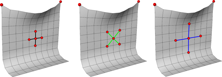
Three families of springs are classically used, each targeting a particular deformation mode:
If only structural springs are used, the network constrains only edge lengths. However, two very different configurations can share the same edge lengths: a square and a flattened rhombus, for example. The fabric can then shear or fold at no cost, which produces unsightly visual artifacts (formation of sharp creases, loss of volume).

Avec des ressorts structurels seulement, le tissu peut se cisailler ou se plier librement à coût énergétique nul.
The addition of shear springs (diagonals) solves the first problem: any shear deformation changes the length of the diagonals and is therefore penalized. The addition of bending springs (two-ring neighbors) solves the second: any folding between three collinear particles changes the distance between the extreme particles and thus costs energy.

Ajout des ressorts de cisaillement (diagonales courtes) et de flexion (voisinage à 2 anneaux) pour rigidifier le tissu.
The stiffnesses \(K_{ij}\) associated with each family are generally different: \(K_{\text{struct}} > K_{\text{shear}} > K_{\text{bend}}\), reflecting the fact that elongation is typically the most energetically costly deformation mode.
Each particle \(i\) of the fabric experiences three types of forces: gravity, a drag force (modeling air resistance, which damps parasitic oscillations) and the sum of the elastic forces exerted by all springs to which it is connected. The total force is written as:
\[ \mathbf{F}_i(\mathbf{p}, \mathbf{v}, t) = m_i \, \mathbf{g} - \mu \, \mathbf{v}_i(t) + \sum_{j \in \mathcal{V}_i} K_{ij} \, \big( \|\mathbf{p}_j(t) - \mathbf{p}_i(t)\| - L_{ij}^0 \big) \, \frac{\mathbf{p}_j(t) - \mathbf{p}_i(t)}{\|\mathbf{p}_j(t) - \mathbf{p}_i(t)\|} \] where :
The elastic term corresponds exactly to the generalized Hooke’s law: its magnitude is proportional to the deviation from the rest length, and its direction is that of the spring. The damping term \(-\mu \mathbf{v}_i\) is essential in practice: without damping, the system would oscillate forever (the springs store elastic energy).
The tissue’s global ODE is written, for each particle:
\[ \forall i, \quad \left\{ \begin{array}{l} \mathbf{p}_i'(t) = \mathbf{v}_i(t) \\[0.5em] \mathbf{v}_i'(t) = \mathbf{F}_i(\mathbf{p}, \mathbf{v}, t) / m_i \end{array} \right. \] For a fabric of \(N \times N\) particles, we obtain a coupled system of \(6 N^2\) scalar equations (3 for the position, 3 for the velocity of each particle), to be numerically integrated at each time step.
Wind forces are modeled simply by adding a term \(\mathbf{F}_i^{\text{vent}}\) to the total force: for example, a constant force directed along a given direction, optionally modulated by procedural noise to simulate gusts, or a term proportional to \(\mathbf{n}_i \cdot (\mathbf{v}_{\text{air}} - \mathbf{v}_i)\) where \(\mathbf{n}_i\) is the local normal of the fabric (allowing the wind to ‘push’ the areas perpendicular to its direction and to slide over the areas parallel to it).
One often neglected point in a first approach is the self-collision of the fabric: springs alone do not prevent it from intersecting itself. Handling it requires testing non-adjacent triangle pairs at each time step (with a broad-phase to stay tractable), then applying a position- or velocity-based response as for spheres — this is one of the main sources of complexity in a robust implementation.
Let us revisit the case of the isolated 1D spring without damping (for which the exact solution is the perfectly harmonic oscillation). If we integrate with explicit Euler, the energy analysis reveals a pathological behavior. The total energy of the system, the sum of kinetic energy and elastic potential energy, equals:
\[ E = \frac{1}{2} m \, v^2 + \frac{K}{2} (p - l^0)^2 \] At the instant \(t^{k+1}\), after an explicit Euler step (\(v^{k+1} = v^k - \frac{K}{m} \Delta t \, (p^k - l^0)\) and \(p^{k+1} = p^k + \Delta t \, v^k\)), we compute the energy:
\[ E^{k+1} = \frac{1}{2} m \left( -\frac{K}{m} \Delta t \, (p^k - l^0) + v^k \right)^2 + \frac{1}{2} K \, (p^k + \Delta t \, v^k - l^0)^2 \] By expanding the two squares and regrouping the terms, we obtain:
\[ E^{k+1} = \underbrace{\frac{1}{2} m \, (v^k)^2 + \frac{1}{2} K \, (p^k - l^0)^2}_{E^k} + \frac{1}{2} \left[ \underbrace{\frac{K^2}{m} (\Delta t)^2 \, (p^k - l^0)^2}_{> 0} \underbrace{- 2 K \Delta t \, (p^k - l^0) \, v^k + 2 K \Delta t \, (p^k - l^0) \, v^k}_{= 0} + \underbrace{K (\Delta t)^2 \, (v^k)^2}_{> 0} \right] \] The two cross terms cancel exactly, but the two squared terms are strictly positive. From this we deduce:
\[ E^{k+1} = E^k + \varepsilon \, (\Delta t)^2, \quad \varepsilon > 0 \] The energy thus increases at each time step by an amount proportional to \((\Delta t)^2\). The result is a systematic divergence: the amplitude of the oscillations grows without bound, and the simulation blows up after some time. Reducing \(\Delta t\) only slows the phenomenon; it does not eliminate it.
This result is qualitatively true for any oscillatory system: Explicit Euler is unconditionally unstable for purely oscillatory ODEs. For the cloth, this translates into particles that escape to infinity after a few seconds of simulation, even with a very small time step. A more sophisticated scheme is needed.
The simplest solution — and the most widely used in computer graphics practice — is the semi-implicit Euler, also known as the Verlet integration (in its position-based formulation). The trick is to use, in updating the position, the new velocity \(\mathbf{v}^{k+1}\) rather than the old \(\mathbf{v}^k\).
For an ODE of the form \(u'(t) = (\mathcal{F}_p(p, v, t), \mathcal{F}_v(p, v, t))\), we write:
\[ \left\{ \begin{array}{l} \mathbf{v}^{k+1} = \mathbf{v}^k + h \, \mathcal{F}_v(\mathbf{p}^k, \mathbf{v}^k, t^k) \\[0.5em] \mathbf{p}^{k+1} = \mathbf{p}^k + h \, \mathcal{F}_p(\mathbf{p}^k, \mathbf{v}^{k+1}, t^k) \end{array} \right. \] which specializes in the classical mechanics case \(\mathbf{p}'(t) = \mathbf{v}(t)\), \(m \mathbf{v}'(t) = \mathbf{F}(\mathbf{p}, t)\) in:
\[ \left\{ \begin{array}{l} \mathbf{v}^{k+1} = \mathbf{v}^k + h \, \mathbf{F}(\mathbf{p}^k, t^k) / m \\[0.5em] \mathbf{p}^{k+1} = \mathbf{p}^k + h \, \mathbf{v}^{k+1} \end{array} \right. \] We can see that the only difference with explicit Euler is the replacement of \(\mathbf{v}^k\) by \(\mathbf{v}^{k+1}\) in the second equation. The conversion of an existing explicit Euler implementation to semi-implicit Euler is therefore trivial, which makes it an excellent first improvement.
// Euler explicite (instable sur les ressorts)
v = v + h * F(p, t) / m;
p = p + h * v_old;     // <-- utilise la vitesse précédente

// Euler semi-implicite (stable)
v = v + h * F(p, t) / m;
p = p + h * v;          // <-- utilise la nouvelle vitesse
By substituting \(\mathbf{v}^k \simeq (\mathbf{p}^k - \mathbf{p}^{k-1}) / h\) into the semi-implicit scheme, one can completely eliminate the velocity from the state:
\[ \mathbf{p}^{k+1} = 2 \, \mathbf{p}^k - \mathbf{p}^{k-1} + h^2 \, \mathbf{F}(\mathbf{p}, t) / m \] This formulation, called Verlet integration in the strict sense, stores only the two most recent positions (not the velocity). It is widely used in molecular dynamics and in some game engines for its simplicity and memory efficiency.
In terms of accuracy, the semi-implicit scheme is first-order in position and velocity (like explicit Euler or implicit Euler), but it has a crucial property: it is conditionally stable for oscillatory systems. The energy no longer diverges; it remains bounded and oscillates around the exact value with a small error. This property is called symplectic: the scheme approximately preserves the energy of a Hamiltonian system (on average over a large number of steps).
The stability condition remains nevertheless constraining: for a spring with stiffness \(K\) and mass \(m\), the time step must satisfy \(h \lesssim 2 / \omega = 2 \sqrt{m/K}\), where \(\omega\) is the natural angular frequency of the spring. For a coupled system like a fabric, it is the largest angular frequency \(\omega_{\max}\) — typically carried by the stiffest springs (often the structural or bending springs) — that dictates the bound. Doubling the stiffness therefore requires dividing the time step by \(\sqrt{2}\), which quickly becomes prohibitive for very stiff fabrics.
In practice, for fabric simulation and moderately rigid mass-spring systems, semi-implicit Euler remains an excellent default choice. When the bound on \(h\) becomes too small, one switches to implicit schemes (implicit Euler, Newmark) which require solving a linear system at each step but allow much larger time steps. This trade-off between cost per step and step size is one of the central questions of physics-based simulation in computer graphics.
The animation of an articulated character — a human, an animal, an imaginary creature — poses problems that do not appear in the rendering of a static scene. The character must be able to assume any pose, without having to manually model each of them, and the deformation of its surface (skin, clothing glued to the body) must naturally follow the movement of the limbs. It must also be possible to specify the animation at an abstract level — « the left foot lands here », « the arm reaches the hand toward this object » — without constraining individually each of the hundreds or thousands of vertices of the mesh.
Two concepts address the bulk of these difficulties. The animation skeleton reduces the character’s pose to a few tens of parameters (the joint rotations), much more manageable than the complete mesh. The skinning defines how the surface deforms as a function of this skeleton, by attaching each vertex to one or more bones. Once these two building blocks are in place, we can drive the animation by forward kinematics — by adjusting the joint angles — or by inverse kinematics — by specifying the positions of the end effectors and letting the solver deduce the angles.
An animation skeleton is a hierarchical structure of frames \(\mathrm{M}_i\) (each composed of a position and an orientation), articulated to one another. The common terminology — borrowed from anatomy even if it deviates from it — distinguishes:
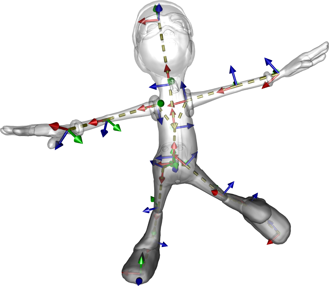
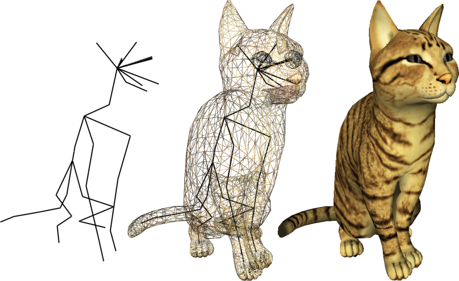
Un squelette d'animation est un ensemble de repères articulés. Il décrit les degrés de liberté du personnage, indépendamment de la géométrie de la peau.
It should be stressed from the outset that this skeleton is not intended to reproduce anatomy: a cat skeleton for animation purposes typically has a few dozen joints, whereas real anatomy comprises hundreds. Its role is to capture the degrees of freedom relevant to posing and movement, while remaining light enough for the animator (or an IK algorithm) to manipulate it in real time.
The rigid skinning is the simplest approach to make the character’s surface follow the skeleton. We attach each vertex of the mesh to a single bone, and apply to it the rigid transformation of that bone: if the bone rotates, the vertex rotates with it; if the bone translates, the vertex translates as well.
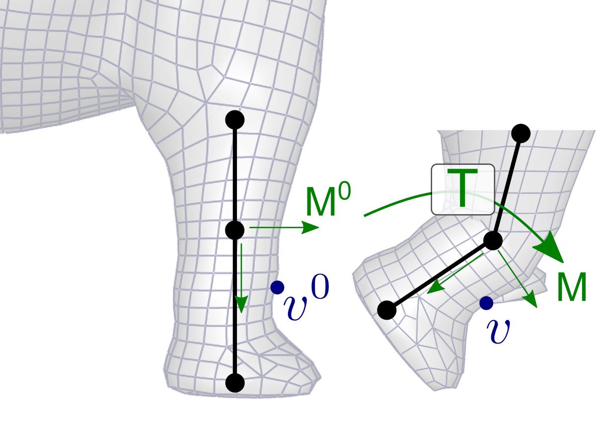

Skinning rigide : chaque sommet est associé à un os, et suit la transformation rigide du repère correspondant.
To formalize this deformation, we introduce the notion of rest pose (bind pose): the reference configuration in which the skeleton and the mesh were initially modeled. Let \(\mathrm{M}^0\) denote the frame of a bone in the rest pose, and \(v^0\) the position of a vertex attached to this bone, expressed in the world frame. When the bone moves to a new frame \(\mathrm{M}\) (during animation), we seek the new position \(v\) of the vertex.
The key idea is that the local coordinates of the vertex, expressed in the bone’s frame, do not change: the vertex is rigidly attached to the bone, so its position relative to the frame is fixed. We thus have:
\[ \mathrm{M}^{-1} \, v = (\mathrm{M}^0)^{-1} \, v^0 \] (the two expressions give the local coordinates of the vertex, which are identical by hypothesis). By multiplying on the left by \(\mathrm{M}\), we obtain:
\[ v = \mathrm{M} \, (\mathrm{M}^0)^{-1} \, v^0 = \mathrm{T} \, v^0 \] where \(\mathrm{T} = \mathrm{M} \, (\mathrm{M}^0)^{-1}\) is the transformation matrix of the bone between the rest pose and the current pose. This matrix is precomputed once per image (for each bone) and then applied to all vertices attached to that bone.
Rigid skinning is easy to implement and yields perfect results on objects that are themselves rigid (an articulated robot, a mechanical crane, an excavator arm). For an organic character, however, it poses, an obvious problem: at the joints, where two bones meet, the transformation changes abruptly from one vertex to the next, creating visible discontinuities. Depending on the bend direction, the mesh tears (on the outside of the elbow) or self-intersects (on the inside).
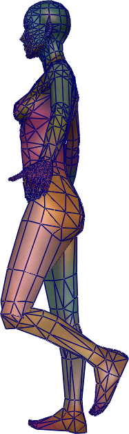
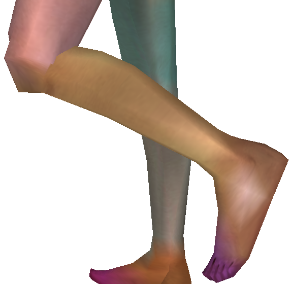
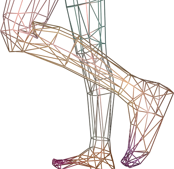
Artefacts typiques du skinning rigide aux articulations : discontinuités, auto-intersections, perte de volume.
The natural idea for solving this problem is to mix the transformations in the vicinity of each joint, rather than abruptly switching from one to the other. This is precisely what smooth skinning does, as presented in the following section.
The Linear Blend Skinning (LBS) is today the standard technique for deforming articulated characters, in cinema as in video games. Its principle is a linear interpolation of the positions computed by the rigid skinning associated with each neighboring bone.

Consider, for example, a vertex located exactly between two bones \(b_1\) and \(b_2\) (halfway along the elbow of an arm, for example). Rather than attaching it to one of the two, we compute two candidate positions — \(p_{|b_1} = \mathrm{T}_1 \, p^0\) via the transformation of \(b_1\), and \(p_{|b_2} = \mathrm{T}_2 \, p^0\) via that of \(b_2\) — and then we take their average:
\[ p = 0{,}5 \, p_{|b_1} + 0{,}5 \, p_{|b_2} = 0{,}5 \, \mathrm{T}_1 \, p^0 + 0{,}5 \, \mathrm{T}_2 \, p^0 = (0{,}5 \, \mathrm{T}_1 + 0{,}5 \, \mathrm{T}_2) \, p^0 \] The final form reveals a remarkable property of LBS: one can average the transformation matrices rather than the positions, and apply the blended matrix to \(p^0\). This allows precomputing a single matrix per vertex per frame, and reusing the same shader code as for rigid skinning.
For the general case of a vertex \(i\) influenced by \(N\) bones, we assign to each bone \(j\) a skinning weight \(\alpha_{ij} \in [0, 1]\) satisfying \(\sum_j \alpha_{ij} = 1\) (partition of unity). The deformed position is then written as:
\[ p_i = \left( \sum_{j=0}^{N-1} \alpha_{ij} \, \mathrm{T}_j \right) p_i^0 = \left( \sum_{j=0}^{N-1} \alpha_{ij} \, \mathrm{M}_j \, (\mathrm{M}_j^0)^{-1} \right) p_i^0 \]
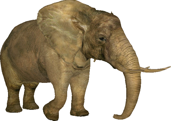
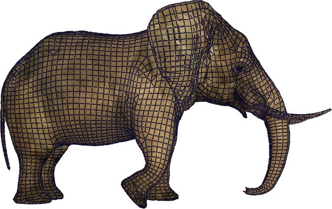
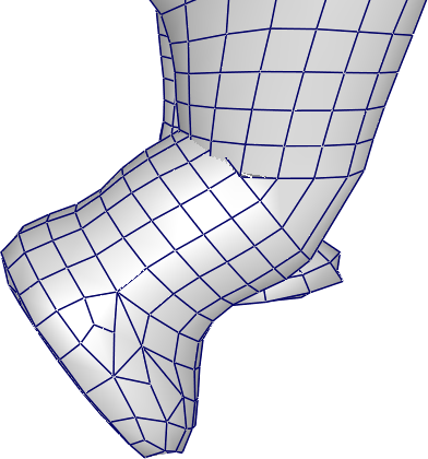
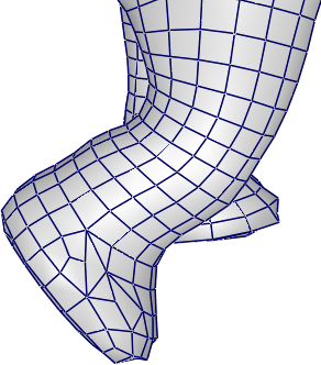
LBS appliqué à un éléphant : la même peau prend différentes poses sans apparition d'artefacts visibles aux articulations.
LBS owes its ubiquity to three properties. Its deformation is intuitive (each vertex follows the visual blend of the bones that influence it). Its shape is controllable by weights — an artist can paint customized weights to locally adjust the behavior. And its cost is very low: for each vertex, it is a weighted average of a few matrices followed by a matrix-vector product, operations perfectly suited to the GPU and executed in the vertex shader. That is why the LBS remains, nearly forty years after its introduction by Magnenat-Thalmann et al. in 1988, the de facto standard in the industry.
LBS nevertheless has known drawbacks — loss of volume at extreme bending (the candy wrapper effect during a 180° rotation), elbow flattening — which have motivated numerous variants (dual-quaternion skinning, example-based methods, cage-based deformation). For the vast majority of common animations, these drawbacks remain acceptable, and the LBS remains the default choice.
The practical question remains: where do the weights \(\alpha_{ij}\) come from? Two approaches dominate.
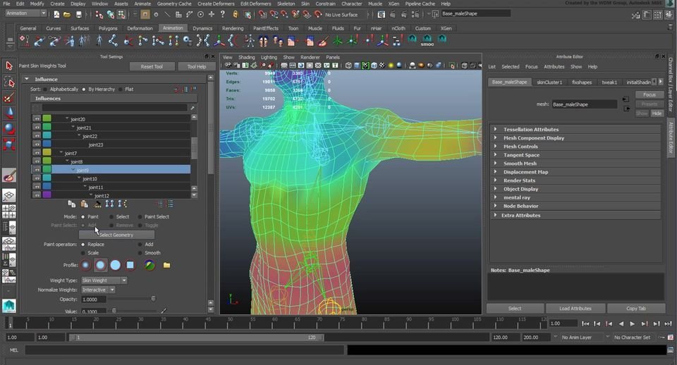
The first approach consists in painting them manually. 3D animation software (Blender, Maya, etc.) enables the artist to visualize the influence of a bone by means of a color gradient on the mesh, and to refine it with a brush. This approach provides the greatest artistic control but requires a lot of time for a complex character.
The second approach automatically computes weights from a geometric heuristic. The simplest is to weight by the inverse of the distance between the vertex and each bone. For two bones \(b_1\) and \(b_2\) at distances \(d_1\) and \(d_2\) from a vertex:
\[ \alpha_1 = \frac{d_1^{-1}}{d_1^{-1} + d_2^{-1}}, \quad \alpha_2 = \frac{d_2^{-1}}{d_1^{-1} + d_2^{-1}} \] Which yields \(\alpha_1 = 1\) when \(d_1 \to 0\) and falls off rapidly as the vertex moves away from \(b_1\). This formula readily generalizes to \(N\) bones.
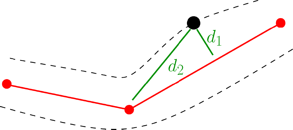
For complex geometries, we prefer methods based on diffusion of a harmonic function over the volume or surface of the character, which take into account the connectivity of the mesh and prevent the weights « pass » through a cavity.
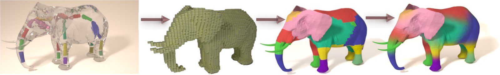
The operation that consists of associating a skeleton and skinning weights (or more generally animation handles) to a static mesh is called rigging. It is typically a distinct step from modeling (the creation of geometry) and animation (the movement of the skeleton), entrusted to a dedicated role in studios.
An animation skeleton is, first and foremost, a hierarchical structure: all the children of a joint inherit its transformation, which reflects the mechanical logic of the body (rotating the shoulder propagates to the elbow, the wrist, and the hand). We thus designate a particular joint as the root of the hierarchy — typically the pelvis for a humanoid — from which all other bones descend via parent-child relationships.
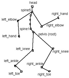
Such a hierarchical representation naturally lends itself to expressing a pose in relative transformations: « the ankle is tilted by 20° relative to the knee », « the forearm forms an angle of 90° with the arm ». It is in this form that poses are stored in the animation files and manipulated by the animators: each joint has its own local rotation, independently of the absolute orientation of the character in the world.

To pass from local transformations to global transformations (used by rendering and skinning), we compose by climbing up the hierarchy. With homogeneous \(4 \times 4\) matrices, the formula is immediate:
\[ \mathrm{M}^i_{\text{global}} = \mathrm{M}^{p(i)}_{\text{global}} \, \mathrm{M}^i_{\text{local}} \] where \(p(i)\) denotes the parent of joint \(i\). If one prefers to separate rotation and translation (a representation useful for interpolating rotations in quaternion form), the composition yields:
\[ R^i_{\text{global}} = R^{p(i)}_{\text{global}} \, R^i_{\text{local}}, \quad t^i_{\text{global}} = t^{p(i)}_{\text{global}} + R^{p(i)}_{\text{global}} \, t^i_{\text{local}} \] The simplest encoding of a skeleton in memory relies on two parallel arrays: one array of local transformations, and an array of indices indicating the parent of each joint (with the convention \(-1\) for the root).

Geometry = [M0, M1, M2, M3, M4, M5]
Parent   = [-1,  0,  1,  1,  0,  4]
An important convention facilitates implementation: if we sort the joints in topological order (each joint appears after its parent in the array), the local → global conversion is performed in a single linear pass:
// local, global : std::vector de structures { rotation r, translation p }
global[0] = local[0];
for (size_t k = 1; k < N; ++k) {
    int parent = Parent[k];
    global[k].r = global[parent].r * local[k].r;
    global[k].p = global[parent].r * local[k].p + global[parent].p;
}
At each iteration, the parent has already been processed, therefore
global[parent] indeed contains the parent’s global
transformation. This sorting convention is respected by most animation
formats (FBX, glTF, BVH), precisely to enable this update in \(O(N)\).
The Direct Kinematics (Forward Kinematics, FK) is the most direct method for specifying an animation: the animator manually sets the angle of each joint, and the positions of the endpoints are deduced by composition. This is the natural approach to orient a specific part of the body — the head, the pelvis, a flag held in the hand — where what matters is the orientation, not a precise target position.
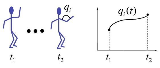
To produce a continuous animation, we define key poses at different moments, and we interpolate the rotations between these poses to obtain the intermediate states. This is where an often-underestimated advantage of FK appears: interpolating a rotation around a joint (for example the elbow) automatically generates a curved trajectory of the end effector (the hand describes an arc of a circle around the elbow). For large movements — a punch, the swing of an arm during walking — this property yields natural trajectories without the animator’s effort.
FK, however, shows its limits as soon as one seeks to impose a precise position on an end effector. If one wants the character’s foot to be placed exactly on a stair step, it is very difficult to adjust the angles of the hip, knee, and ankle to achieve the correct result — not to mention that the slightest modification propagates to the entire chain. This is precisely the role of inverse kinematics.
The Inverse Kinematics (Inverse Kinematics, IK) resolves the dual problem of FK. Rather than specifying the joint angles and calculating the position of the endpoints, one specifies the position (and possibly orientation) of a final effector — a point on the skeleton designated as the target, typically a hand, a foot or the head — and we seek the joint angles that allow reaching this position.
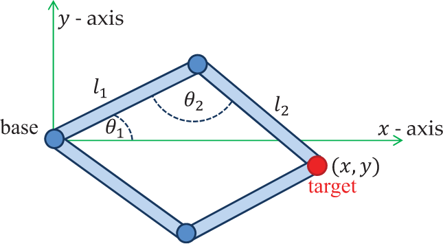
This is the natural animation mode for locomotion (the feet must land at precise positions on the ground) and for object manipulation (the hand must grab a precise object in the scene). Mathematically, letting \(p_k\) denote the position of the end-effector at the end of the chain, we have the relation:
\[ p_k = p_0 + \sum_{i=0}^{k-1} l_i \, R_i \, u_i \] where \(p_0\) is the root position, \(l_i\) the length of bone \(i\), \(u_i\) its reference direction, and \(R_i\) a parameterized rotation matrix (for example by Euler angles, an axis-angle, or a quaternion — the choice of parameterization influences the solver but not the formulation). The forward problem \(p_k = f(\theta_i)\) is straightforward to evaluate; it is the inverse \(\theta_i = f^{-1}(p_k)\) that is difficult.
Several properties make this inversion nontrivial. The function \(f\) is nonlinear (it involves compositions of rotations); there may exist several solutions (the elbow can often reach the same position « over » or « under »), there may be none (the target is out of reach), and the admissible solutions may exhibit discontinuities as the target moves (the elbow abruptly switches from one position to another). Consequently, in general no closed-form formula exists: one must resort to specialized solvers.
The special case of a two-link chain (shoulder + elbow to the hand, or hip + knee to the foot) admits a simple analytic solution, which can be derived by trigonometry. By considering the plane defined by the chain and the target, and denoting \(l_1, l_2\) the lengths of the two bones and \((x, y)\) the target position relative to the shoulder, we obtain:
\[ \cos(\theta_1) = \frac{l_1^2 + x^2 + y^2 - l_2^2}{2 \, l_1 \, \sqrt{x^2 + y^2}}, \quad \cos(\theta_2) = \frac{l_1^2 + l_2^2 - (x^2 + y^2)}{2 \, l_1 \, l_2} \] (the first line gives the angle θ1 of the first bone with respect to the shoulder→target direction, the second the internal angle θ2 between the two bones, by applying the Law of Cosines to the triangle formed). The sign of the sine corresponding to θ2 gives the two solutions (elbow « above » or « below »), to be chosen depending on the context (typically by continuity with the previous pose).
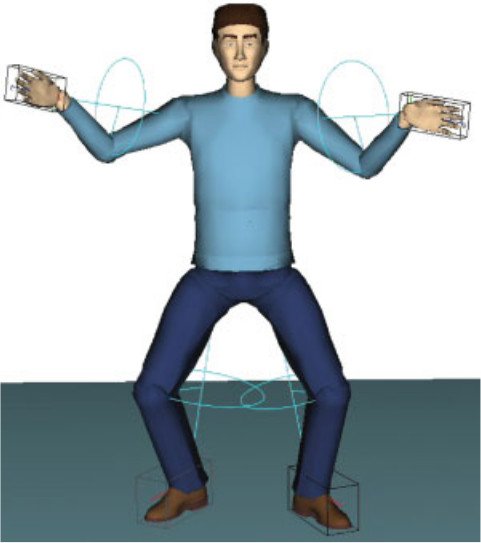
This particular case is sufficiently common (almost all human or animal limbs reduce to two-bone chains: arm, leg) that we implement it as a special case in animation engines, reserving numerical solvers for longer chains or for additional constraints (imposed orientation of the hand, for example). Several works extend the analytic approach to broader configurations by imposing specific parameterizations (Tolani 2000, Kallmann 2008), but their scope remains limited to very specific morphologies.
For more complex chains, we locally linearize the problem. The Jacobian matrix \(\mathrm{J}\) relates a small variation of the angles \(\Delta \theta\) to the corresponding variation of the end-effector position \(\Delta p\):
\[ \mathrm{J} \, \Delta \theta = \Delta p \] The system is not square in general (\(\mathrm{J}\) typically has more columns than rows: there are more joint angles than target coordinates, which corresponds to the kinematic redundancy). We solve it by pseudo-inverse:
\[ \Delta \theta = \mathrm{J}^+ \, \Delta p, \quad \mathrm{J}^+ = \mathrm{J}^T \, (\mathrm{J} \, \mathrm{J}^T)^{-1} \] where \(\mathrm{J}^+\) is the Moore-Penrose pseudoinverse, which among all the solutions \(\Delta \theta\) selects the one with minimal norm (the smallest joint movement). It can also be computed via the singular value decomposition (SVD) :
\[ \mathrm{J}^+ = \mathrm{V} \, \Sigma^+ \, \mathrm{U}^T, \quad \Sigma^+_{ii} = \begin{cases} 1/\sigma_i & \text{si } \sigma_i \ne 0 \\ 0 & \text{sinon} \end{cases} \] In the vicinity of singularities (configurations where the chain is stretched to its maximum, for example), some singular values \(\sigma_i\) tend to zero and the pseudo-inverse explodes, producing erratic joint movements. We stabilize the solver then by the Damped Least Squares method (Damped Least Squares):
\[ \Delta \theta = \mathrm{J}^T \, (\mathrm{J} \, \mathrm{J}^T + \lambda^2 \, \mathrm{I})^{-1} \, \Delta p \] The parameter \(\lambda\) is a trade-off: too small, the solver remains unstable near singularities; too large, it converges slowly away from the target. It is typically adjusted adaptively according to the smallest singular value. Once \(\Delta \theta\) is obtained, we increment the angles, we re-evaluate the error \(\Delta p\) toward the target, and we iterate until convergence — this is the spirit of Newton’s methods applied to the IK.
Jacobian-based methods are accurate but costly (solving a linear system at each iteration). For real-time requirements — typically video games — simpler heuristic methods are often preferred to them. The best-known one is the cyclic coordinate descent (Cyclic Coordinate Descent, CCD), introduced in the context of animation by Jeff Lander in 1998.
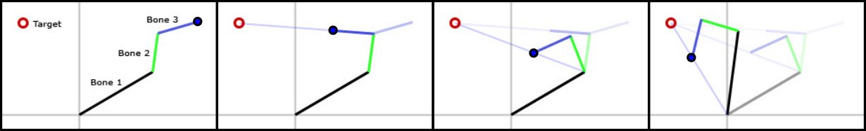
The algorithm operates joint by joint, starting from the last one (just before the end effector) and moving up toward the root. At each joint \(j^i\), we compute the rotation that best aligns the segment (joint, end effector) with the segment (joint, target), and apply it. Once all joints have been processed, the end effector is closer to the target but probably not on it; we then start a new iteration from the end and continue until convergence (typically a few tens of iterations).
CCD has several advantages: it requires no matrix inversion, it is trivial to implement (a few dozen lines), and it converges in a predictable manner (useful to guarantee a cost per frame bounded in a game engine). Its convergence, however, is linear (vs quadratic for Newton), which makes it slow when far from the target, and it tends to bias rotations toward the end effector (the joints near the root move little), which can produce poses that look unnatural.
FABRIK (Forward And Backward Reaching Inverse Kinematics), introduced by Aristidou and Lasenby in 2011, is a more recent heuristic approach that solves IK solely by operations on the positions of the joints (without explicitly manipulating the rotations), while respecting the lengths of the bones.
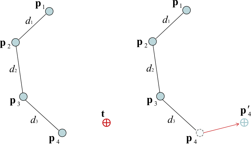
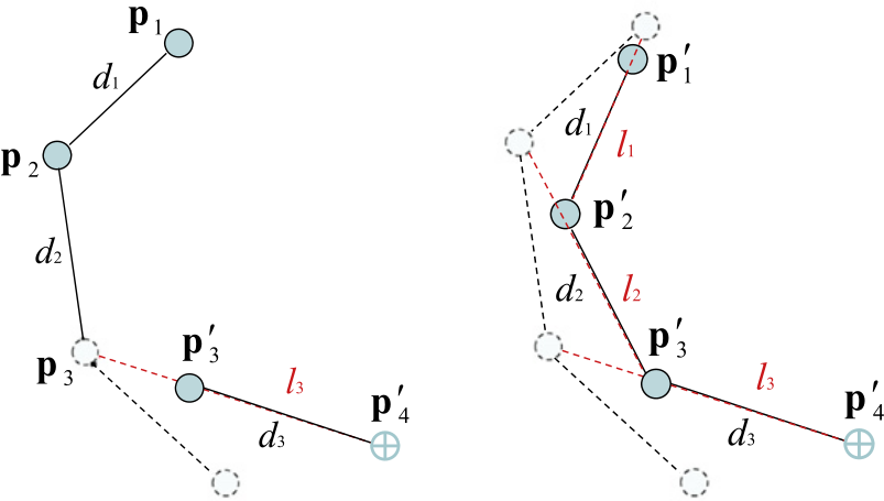
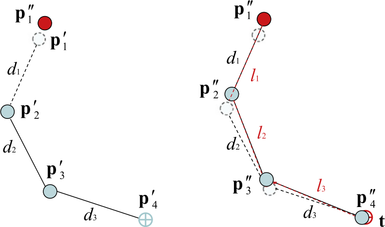
FABRIK : configuration initiale, passe avant (effecteur amené sur la cible, longueurs propagées vers la racine), passe arrière (racine ramenée à sa position d'origine, longueurs propagées vers l'effecteur).
Each iteration consists of two passes. The forward pass first moves the end effector to the target position, then climbs the chain by repositioning each joint on the line connecting its successor to the new position of the child, at the distance imposed by the bone length. At the end of this pass, the lengths are respected and the end effector is at the target — but the root has moved, which is unacceptable. The backward pass then starts from the root, restores it to its original position, then descends the chain by repositioning each joint on the line connecting its predecessor to the new position of the parent. At the end of this second pass, the root is back but the end effector has moved.
More formally, by denoting \(p_0, p_1, \ldots, p_N\) the positions of the joints (with \(p_0\) the root and \(p_N\) the end effector), \(l_i = \|p_{i+1} - p_i\|\) the imposed lengths, and \(t\) the target, the algorithm is written as:
Entrées : positions p[0..N], longueurs ℓ[0..N−1], cible t,
          tolérance ε, nombre max d'itérations k_max

p_racine <- p[0]
L <- ℓ[0] + ℓ[1] + ... + ℓ[N−1]

# Cas 1 : cible hors de portée — étirer la chaîne en ligne droite vers t
si ‖t − p[0]‖ > L alors
    pour i de 0 à N−1 faire
        λ <- ℓ[i] / ‖t − p[i]‖
        p[i+1] <- (1 − λ) · p[i] + λ · t
    retourner p
fin si

# Cas 2 : cible atteignable — itérer passes avant et arrière
répéter au plus k_max fois
    si ‖p[N] − t‖ < ε alors retourner p

    # Passe avant : amener l'effecteur sur la cible
    p[N] <- t
    pour i de N−1 à 0 faire
        λ <- ℓ[i] / ‖p[i+1] − p[i]‖
        p[i] <- (1 − λ) · p[i+1] + λ · p[i]

    # Passe arrière : remettre la racine en place
    p[0] <- p_racine
    pour i de 0 à N−1 faire
        λ <- ℓ[i] / ‖p[i+1] − p[i]‖
        p[i+1] <- (1 − λ) · p[i] + λ · p[i+1]
fin répéter

retourner p
The heart of the algorithm comes down to two lines per step: we compute a coefficient \(\lambda = l_i / r\) (where \(r\) is the current distance between two consecutive joints), then we move the joint by a simple linear interpolation that restores the length \(l_i\). It is this simplicity — no matrix to invert, no angle calculation, no trigonometric resolution — that makes the method so powerful: each iteration costs \(O(N)\) vector operations, and the algorithm vectorizes well on GPUs.
Once the positions \(p_i\) are obtained, we derive the joint rotations by cross product or by direct construction of an orthonormal frame (relying on the axis of the previous bone and any orientation constraints), before reapplying the LBS on the mesh. For branched chains (the full humanoid skeleton with two arms and two legs), we treat each sub-chain independently and then reconcile the positions at the shared joints (shoulders, hips), in a few additional iterations. Angle constraints are handled in the forward or backward pass by projecting the calculated position onto the cone allowed by the joint limits.
In practice, FABRIK converges in only a few iterations, produces poses that look visually natural, and generalizes well to joint constraints (angle limits). It has become one of the most used IK solvers in modern game engines (Unreal Engine includes it directly under the name Two Bone IK / FABRIK Solver).
The techniques discussed here — FK, analytical IK, Jacobian-based methods, CCD, FABRIK — cover the essentials of what an animation engine uses on a daily basis. Beyond that, more advanced approaches (motion capture combined with retargeting, blending of motion graphs, physics-based controllers for locomotion) allow producing animations even more natural from real data or physically simulated rigs — but they all rely, at some point, on the skeleton and the skinning described in this chapter.