3/7
3. Keyframe Interpolation
Position-keyframe
Linear interpolation
-
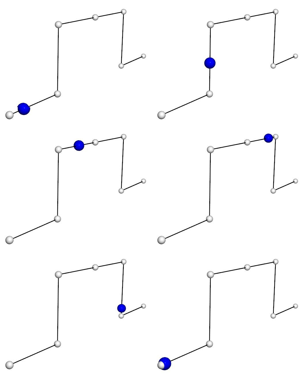
Set the code to run the scene from exercises/02_interpolation/interpolation_position.hpp (#define EXERCISE_INTERPOLATION_POSITION)
-
This code compute the linear interpolation between keyframes (displayed as white spheres) defined by a position and a time. The interpolated value is displayed by the moving blue sphere.
Note that time loop can be manually adjusted using the GUI.
-
Observe how the linear interpolation is computed in this example.
Cubic Cardinal Spline interpolation
-
Code a function taking as arguments
-
The current time \(t\)
-
Four keyframe position \(p_0,p_1,p_2,p_3\)
-
Four keyframe time \(t_0, t_1, t_2, t_3\)
-
The curve tension and returns the value \(p(t)\) obtained as cubic cardinal spline interpolation.
-
The C++ signature of your function may be
vec3 spline_cardinal(float t,
                     const std::array<vec3,4> P,
                     const std::array<float,4> T,
float tension);-
Use this function to change the linear interpolation of the blue sphere position to a cardinal spline. Take care to stay within the valid interval of time.
-
Adapt your keyframe data to ensure that the interpolation starts at the first visible point, and stop at the last visible point.
-
Display the trajectory followed by your interpolated position. (Your may use the curve_drawable object).
-
Test your interpolation on different data inputs and different curve tensions. You may adapt the keyframe time such that the time between two keyframe position is given by the distance between the samples.
Blend Shapes
Character’s face data
-
Consider the scene from exercises/02_interpolation/blend_shape.hpp.
This time the code loads a set of faces of a character as meshes. No interpolation is performed between the different poses. Note that the body of the character is static, and is stored as another mesh.
-
Adapt the code to enable cardinal spline interpolation. Compare the visual result between linear interpolation and cardinal spline interpolation. Note that you may adapt the order of the index_order variable to adapt the motion of the character’s face. In real case scenario such as speaking animation, this order can be adapted dynamically.
-
Which normals are used during the animation ? Can you propose a solution allowing to have more accurate normals ?
Horse gallop data
-
Change the input data to load the running horse data/horse-gallop.
-
You may want to adapt the time of the keyframe such that the entire animation runs in about 5s.
-
You can load the positions from mesh files using the following codes
-
for(size_t k=0; k<N; ++k)
{
    const std::string filename = "data/horse/horse-gallop-"+zero_fill(std::to_string(k+1),2)+".obj";
    keyframe_position.push_back(mesh_load_file_obj_read_vertices(filename));
}-
Observe the artifact to to vertex interpolation when the leg of the horse changes quickely of orientation.
-
Display the trajectory followed by a vertex (e.g. vertex at index 1792). Observe the difference between linear and cubic spline vertex trajectory.
Rigid bodies interpolation
-
Consider the scene from exercises/02_interpolation/interpolation_rotation.hpp.
-
The code interpolates a frame using linear interpolation on matrices.
-
Implement quaternion interpolation, and compare the resulting interpolation for different rotation parameters.
-
Display the trajectories of the frame vector extremities.
If you have time
-
Implement Euler angle interpolation, and compare the trajectory followed by the frame with respect to quaternion interpolation.
-
You may consider the following conversion between a rotation matrix \(R\) and a \(R_z(\theta_3)\,R_y(\theta_2)\,R_x(\theta_1)\) Euler angle representation
-
\(\tan(\theta_1)=R_{yz}/R_{zz}\)
-
\(\tan(\theta_2)=-R_{xz}/\sqrt{R_{xx} ^ 2+R_{xy} ^ 2}\)
-
\(\tan(\theta_3)=(\sin(\theta_1) R_{zx}-\cos(\theta_1) R_{yx})/(\cos(\theta_1)R_{yy}-\sin(\theta_1) R_{zy})\)
-
-
-
Apply your interpolation on a mesh to model the motion of a moving object.